WIXLIB

20NormalizedSpeedupspeedup 00300400500Applied optimizationsequences sortedby increasing actual speedupOptimizationSequences600Figure 1. This graph shows actual speedups (solid line) for 600 sequencesapplied to the program 2MM. We also show predicted speedups (dottedline) for those same sequences obtained from a prediction model that isnot trained with 2MM and that uses our graph-based characterization. Thex-axis shows optimization sequences sorted by increasing order of actualspeedup, and the y-axis shows speedup obtained after applying a sequenceover some baseline (ICC -fast). Triangles correspond to the top 5 predictedsequences, and circles correspond to next best 5 predicted sequences.overview of our solution giving more details of how we constructand use the prediction models. We explain our experiment setup inSection 4 and demonstrate results and present analysis in Section5. In Section 6, we explain and compare it to related work. Section7 presents our conclusions and future work.2.Characterizing the ProgramCompiler researchers have proposed to use machine learning models to focus search on beneficial areas of the optimization searchspace [6, 10, 11, 14, 20, 25]. An important step in using these models is to characterize (or construct features for) the programs beingoptimized. Finding the “right” set of features and a good representation for this information is one of the most challenging, andprobably the least automatable, part of the process.Compiler researchers have used fixed-length representations ofthe program’s source code features and intermediate representation [6, 20, 25]. These representations are straight-forward to extract from a program and can be collected during compilation time.However, these representations are less expressive and are oftenout-performed by more expensive dynamic techniques. Other researchers have proposed using dynamic characterizations of programs; however, techniques (e.g., performance counters [10] andreactions [15, 27]) are expensive and require running the program,which limits their practical use.In this section, we motivate the applicability of using the program’s intermediate representation as unstructured data as input formachine learning for finding good optimization sequences.2.1Different Ways to Characterize the ProgramProgram characterization techniques can be grouped into two categories: static or dynamic methods. The benefit of using a staticcharacterization is that we do not need to run a program. We cancapture these features during the compilation process or by parsingthe source code itself. Previous work on static features has focusedmainly on collecting source code features, such as instruction mix,loop nest depth, etc [6]. Additionally, there has been work on collecting simple summary statistics derived from a program’s intermediate representation, e.g., number of nodes and edges, numberof phi nodes, etc. [16]. Previous work has put this static information into fixed-length vectors, which is essential for traditional supervised learning techniques. However, summarizing this data intofixed-length vectors causes vital information to be lost, such as thecontrol flow through the program.More recently, researchers have looked into characterizing programs using dynamic information, e.g., using performance counters or optimization reactions. Using performance counters, we cancollect multiple characteristics of the running program, such as thebehavior of the cache at each level, number of stall cycles, or themix of different instructions executing, etc. Another method of dynamically characterizing a program is through reactions. Here, werecord the performance impact from a fixed set of different optimization sequences [9, 15]. Thus, we run a program K number oftimes by optimizing it with K different optimization sequences, andthen obtain different speedups for each sequence. These reactionsare used to characterize the program. These dynamic techniqueshave been shown to empirically out-perform static features. However, collecting dynamic information requires running the programat least once and in many cases multiple times to collect these features.In this paper, we propose a novel technique to characterize aprogram using its graph-based intermediate representation (IR). Inparticular, we use the program’s control flow graph (CFG) as thebasis for our graph-based characterization. We also include in thischaracterization information about each instruction at each CFGnode. We convert this characterization into a format that can be fedinto an adapted machine learning algorithm. This is a static characterization and therefore does not require running the program. Themain difference between our technique and previous static techniques is that we encode the topology of the program’s IR intoour characterization. Given this novel characterization, we can produce models that predict optimization sequences that out-performsequences predicted by models using other characterization techniques. We also experimented with other graph-based IRs for program characterization, and we present these results in Section 5.3.Figure 1 shows the predictions for one program from a modelthat uses our graph-based characterization technique. The solid lineshows actual speedup (sorted) optimizing 2MM from the PolyBench suite [3] with random optimization sequences. We randomlygenerated 600 different optimization sequences consisting of different loop/parallelization transformations from the PoCC sourceto-source compiler [2], and we used the ICC compiler with option -fast as the backend compiler to produce an executable fromthe optimized output source code of PoCC. To obtain predictionsfor a model that uses our graph-based characterization, we performed leave-one-out cross-validation to construct a model. Weconstructed the model by training it with the PolyBench programsand by leaving out the benchmark 2MM. Our training data consisted of each program’s graph-based CFG characterization, theabove mentioned 600 optimization sequences, and the speedupsobtained from these sequences. We constructed our models usingsupport vector machines (SVM). We discuss training of our models more thoroughly in Section 3.We observe in Figure 1 that the predicted speedup follows thetrend of the actual speedup similarly although not perfectly. Thismeans there is a high probability that we will get a performanceimprovement by using a sequence (x-value) with a high predictedspeedup (y-value). If we look closer at the top 10 predicted sequences and their predicted y-values (marked by blue triangles andpurple circles in the figure), these sequences are among the best sequences in terms of their actual speedup. In particular, the best predicted sequence from CFG model is the actual best sequence, whichmeans we achieve a speedup of around 19 . In contrast, when wetrain a model for the same machine, but use performance counters

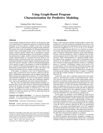
instead of our CFG characterization, we only achieved around 4 ifwe use the best predicted optimization sequence. This preliminaryexperiment shows the potential of using a graph-based representations to characterize programs for predictive modeling.Category of PCsList of PCs selectedCache Line AccessCA-CLN, CA-ITV, CA-SHRL1-DCA, L1-DCH, L1-DCM, L1-ICA, L1-ICH,L1-ICM, L1-LDM, L1-STM, L1-TCA, L1-TCML2-DCA, L2-DCM, L2-DCR, L2-DCW, L2-ICA,L2-ICH, L2-ICM, L2-LDM, L2-STM, L2-TCHL2-TCR, L2-TCW, L2/L3-TCA, L2/L3-TCMBR-CN, BR-INS, BR-MSP, BR-NTK,BR-PRC, BR-TKN, BR-UCNDP/FP/SP-OPS, FDV/FML/FP-INSHW-INT, RES-STLTLB-DM, TLB-IM, TLB-SD, TLB-TLTOT-CYC, TOT-IIS, TOT-INSLD-INS, SR-INSVEC-DP, VEC-INS, VEC-SPLevel 1 CacheLevel 2 & 3 CacheProgram Features (P)Optimization Sequence (O)Branch Related.Floating PointInterrupt/StallTLBTotal Cycle/Insts.Load/Store Insts.SIMD Insts.Table 1. Performance counters (PC): We collected 56 different perforOutput: predicted speedup ofgiven sequence O over baselinemance counters available using PAPI library to characterize a programft1ft2ft3ft4ft5ft6ft7ft8ft9ft10Figure 2. Speedup Predictor3.Automatically constructing a modelThis section describes our prediction model and a detailed description of the different characterization methods we evaluated. We alsogive an explanation of the machine learning algorithm used for ourgraph-based characterization techniques.3.1Speedup Prediction ModelThe prediction model used in this paper is shown in Figure 2. Thismodel has been used in recent work [9, 13, 22] to predict goodoptimization sequences for various different compilers. We referto this model as the speedup predictor because it takes as input aprogram’s characterization (P) and an optimization sequence (O),and it outputs the predicted speedup over some baseline for thatoptimization sequence. In this paper, we use the baseline of PoCCwith no optimization and the backend compiler with its most aggressive setting -fast for ICC and -O3 for GCC). We evaluate ourdifferent characterization methods using the same set of optimization sequences O and build a different speedup prediction modelfor each different characterization method.We evaluate our different models (characterization methods) byusing them in two different scenarios. First, we evaluate them in anon-iterative scenario, where we use only the best predicted optimization sequence from each model. This is the typical scenario,in which a developer uses a compiler. Second, we evaluate thedifferent models in an iterative scenario, where we optimize ourprograms with the N-best predicted optimization sequences, andwe report the speedup obtained by the sequence giving us the bestspeedup. For this paper, we used N 5 since we observed only agradual performance improvement after 5 sequences.3.2Program characteristicsWe collect four different kinds of program features (shown in Figure 4.) to evaluate our different program characterization techniques.Performance Counters (PC) We collect all PC events availableon our target architectures including data/instruction cache behavior, TLB, instruction types, etc. The full list of PCs used in thispaper are shown in Table 1, and all values are normalized by total number of instruction in a given architecture. To collect the PCinformation, we run the program 56 times collecting one counterduring each run of the program. Note that we can collect countersusing multiplexing, but this may introduce noise. The full list ofcounter events used are shown in Table 1, and we show the processof collecting PC information on the top-left of Figure 4.Number of InstructionsNumber of Add instructionNumber of Sub instructionNumber of Mult instructionNumber of Div instructionNumber of Load instructionNumber of Store instructionNumber of ComparisonsNumber of Conditional BranchesNumber of Unconditional BranchesTable 2. Control Flow Graph (CFG): We collected 10 different featuresfor each node (basic block) in CFG. We used MinIR to collect this information.87Feature vector for each node1917621618101: 1,0,0,0,0,0,0,0,0,1 2: 2,0,0,0,0,0,1,0,0,1 3: 8,2,0,1,0,3,1,0,0,1 16: 2,1,0,0,0,0,0,0,0,1 17: 2,0,0,0,0,0,0,1,1,0 18: 1,0,0,0,0,0,0,0,0,1 54151114313Topology of CFG1- 62- 43- 4 16- 1717- 1017- 1812Figure 3. This figure depicts the CFG characterization for 2MM, one ofPolyBench programs. We did not include start and exit nodes inCFG since these nodes are empty (do not include instructions).Reactions We randomly selected a small set K of different optimizations sequences and collect the performance impact for eachof these sequences on each program. The performance impact(speedup or degradation) of these sequences serves as a signaturefor a specific program and are used as input to a prediction model.We used K 5 for this paper. We show the process of collectingthese reactions on the top-right of Figure 4.Source Code Features (SRC) We depict the process of extractingsource code features from programs on the bottom-left of Figure4. We collect different source code features from the MilepostGCC [16] framework. It provides different static features includingproperties of the different instructions and variables used in each

Performance CountersUnderlying ArchitectureK Reactions1MK.1N-1M Performance countersfor N-1 programsSource CodeN-1N-1 programs.K Reactions for N-1 programsN-1N-1MinIRbb3bb4bb5N-1 programsbb6CFG topology and feature ofeach node for N-1 programs.R Source code featuresfor N-1 programsbb2N-1.Feature vector of eachnode.bb1Featureof each bbbb vector.1bb6. .bb1bb.6CFGbb6.CFGTopologybb1- bb2,Topologybb1- bb2,bb3CFG Topologybb3- bb3bb5bb1bb2- bb2bb2,- bb5bb2.- .bb5bb5 - bb6. bb5- bb6bb5 - bb61bb1.N-1.11R.MilepostGCC.11N-1 programsKGraph-based - CFG1N-1.1BackendCompiler.N-1N-1 programs.N-111.BackendCompilerUnderlying ArchitectureK Opt. Seqs.11Figure 4. Collecting Different Program Characterizationsfunction as well as different summary statistics pertaining to basicblocks and edges. We used 34 features from Milepost GCC, whichwere all the relevant features for our programs, i.e., we removedfeatures that were always zero for all our programs.Graph-based characterization (CFG) We show the process ofextracting our graph-based characterization on the bottom-right ofFigure 4. We use MinIR [1] to extract control flow graphs fromeach of our programs. Before generating our CFGs, we run SSAon the programs to give us the property of having one definitionfor each variable. From the CFG, we generate graph-based characterization, which includes 1) a feature vector for each basic blockin the CFG as shown in Table 2 and 2) a list of directed edges inthe graph. MinIR can also be used to extract other graph-based IRs,including the dominator tree, def-use-chain, etc. We describe a preliminary investigation using other graph-based IRs in Section 5.3.Figure 3 shows an example of the CFG of the 2MM program andthe extracted graph-based characterization from the graph. Notethat an important difference between this characterization and previous static characterizations is the presence of topological information of the graph, which is used by an adapted machine learningalgorithm. Also, we collect information per basic blocks, not justa summarization across the entire function, thus providing morefined-grained information to the learning algorithm.OptimizationUnrolling FactorLoop FusionLoop TilingParallelizationVectorizationValue Used0 (no unrolling), 2, 4, 8nofuse, maxfuse, smartfuse1 (no tiling), 32on, offon, offon optimizing loops, thus our search space consists of different looptransformations and different level of parallelism, including threadlevel and instruction-level parallelism. We exhaustively generatedall optimization sequences from this optimization space giving amaximum of 600 optimization sequences, and we evaluate each sequence on our benchmark suite. We collected the speedup obtainedfor each optimization sequence over the baseline of applying noPoCC optimizations. The process of collecting speedups for eachsequence on each program is shown in Figure 5(a). The characterization of each program along with the optimization sequences andtheir corresponding speedups on each program are used to constructthe training data.Constructing the Model Once the training data is constructed, itcan be fed to a learning algorithm that will automatically induce aprediction model as shown in Figure 5(b). We used support vectormachines (SVMs) [23] to construct our predictive models. SVMsare a class of machine learning algorithms that can be used for bothclassification and regression. SVMs use kernel functions to transform the training data into a different, linearly-separable featurespace, and then a linear classifier is constructed that separates thepoints into multiple classes.Using the Model for Unseen Program Figure 5(c) depicts howthe model is used on an unseen program to get predictions of theoptimizations that will work best for that program. We order thepredicted speedups to determine which sequence is predicted best,and apply it to the unseen program. We train our models usingleave-one-out cross-validation, i.e., given N programs, and we traina model on N-1 programs and test the model on the Nth programleft out.Table 3. List of optimization used in this paper. For loop fusion and3.4tiling, our optimization sequences directed which loops to fuse and/or tile.If parallelization is turned on, we parallelize the outer loop. If vectorizationis turned on, we vectorize the inner loop.The use of kernel functions is very attractive because the inputdata does not always need to be expressed as feature vectors. Inour control flow graphs, we would like SVMs to perform structuralcomparisons between different graphs. Note that we cannot simplyflatten this information into feature vectors, because this would remove important information about the structure of the graphs. Suchinformation is useful because it allows the learning algorithm to effectively capture the similarities between two different programs.3.3Building and Using a Prediction ModelCollecting Speedup over Baseline Table 3 gives a list of the optimizations used to create our optimization search space. We focusGraph-based SVM Kernels

Baseline.N-1Opt. SeqsBackendCompiler1.N-1.N-1. . .1.1. .1Opt. seqs and their speedupover baseline for N-1 programsProgram featuresfor N-1 programsN-1.Opt. SeqsN-1 Machine Learning Algorithm.Opt. seqs and their speedupover baselinefor N-1 programsGenerated modelfor a given machine(a) Collecting Speedup over BaselineNth Program(one left out)Extractprogramfeature.(b) Constructing the ModelSame type of feature that we used tobuild a prediction model.Predicted speedupfor each sequence.Optimization Sequences(c) Using the Model for Unseen ProgramFigure 5. This figure depicts how we construct and use our prediction models. This process uses leave-one-out cross validation with N programs. We collectspeedup over baseline for N-1 programs from each sequence in optimization search space as shown in (a). Then, we construct the model from the program’scharacterization, the optimization sequences, and their corresponding speedups (b). We use the model on an unseen program by collecting the program’scharacterization. We then feed this characterization along with the optimization sequences, and the model gives us predicted speedups for those sequences (c).Thus, we are interested in kernel functions that can take discretestructures data as inputs, e.g., control flow graphs.Along these lines, a family of convolution kernels [18] hasbeen introduced as a general framework for building kernels overdiscrete structures. This general framework is based on the idea ofthe decomposition of objects into sub-parts in such a way that akernel function for a pair of objects can be defined as a convolutionof kernel functions defined over their sub-parts. Simple closureproperties of valid kernel functions (positive semi-definite) allowthe definition of kernels in this way. This finding has made greatimpact, and defining kernels for discrete structures has become animportant topic in machine learning [8, 17, 24, 28]. By changingthe decomposition, several types of kernels for graphs have beenproposed so far, including shortest paths, walks, sub-trees, andcyclic patterns.Among all recent developments, graph kernels based on shortestpaths [7] are a remarkable class of kernel functions. They retain expressivity while comparing graphs at acceptable polynomial time.This class of kernels is also attractive because of their wide applicability. Contrary to other graph kernels, shortest path graph kernelscan deal with labeled graphs, where the nodes and edges can belabeled by real values.Shortest Path Graph Kernel Roughly speaking, the basic ideaof a shortest path graph kernel [7] is to quantify the number ofcommon shortest paths in two input graphs. To this end, prior tothe kernel computation, the original graphs must be transformedinto shortest path graphs. Given a graph G hV, Ei, its shortestpath graph is denoted by Gsp hV 0 , E 0 i, where V 0 V andnodes in V 0 are connected by edges e0 (u0 , v 0 ) if there is a pathCFG1Shortest Path gure 6. The control flow graph for GESUMMV and its corresponding shortest-path graph. Note: We choose the simplest CFG from the PolyBench benchmark suite so that the shortest-path graph might be readable.between nodes u and v in the original graph. Edges are labeled withthe length of the shortest distance between u and v in the originalgraph. This transformation can be performed using any all-pairsshortest path algorithm. In particular, we use the Floyd-Warshallalgorithm because it is straightforward and has time complexityof O(n3 ). An example of an original CFG and its correspondingshortest-path graph is shown in Figure 6.Once the original graphs G1 and G2 are transformed into shortest path graphs, the shortest path graph kernel function for a pair

of graphs Gsp1 hV1 , E1 i and Gsp2 hV2 , E2 i is defined asfollows:X Xkwalk (e1 , e2 )Ksp (G1 , G2 ) e1 E1 e2 E2where kwalk is a kernel function for comparing two walks. Awalk includes an edge and its two end nodes. Let e1 be the edgeconnecting nodes v1 and w1 , and e2 be the edge connecting nodesv2 and w2 , then kwalk is defined as:kwalk (e1 , e2 ) knode (v1 , v2 ) · kedge (e1 , e2 ) · knode (w1 , w2 )where knode is a kernel function for comparing two nodes. Onceour control flow graphs have feature vectors at every node, we usethe well-known Gaussian kernel [23] for calculating knode . On theother hand, kedge is a kernel function for comparing two edges. Weuse a Brownian bridge kernel [23] that returns the highest valuewhen two edges have identical length, and 0 when the edges differin length more than a constant c1 as shown below:kedge (e1 , e2 ) max(0, c weight(e1 ) weight(e2 ) )4.Experimental SetupThis section describes our experimental setup, including the machine configurations and compilers we used. We evaluated eachcharacterization technique on two different machines: a Nehalem2-socket 4-cores Intel Xeon 5620 (16 H/W threads) with 12MBL3 cache and a Q9650 4-cores Intel Core 2 Quad Q9650 4 H/Wthreads) with 12MB L2 cache. Our optimization search space camefrom the PoCC source-to-source polyhedral compiler [2]; therefore, we needed a backend compiler to produce executable codefrom our optimized codes. We experimented with two back-endcompilers for each machine: GCC and ICC. We used GCC V4.5and ICC V11.0 for the Nehalem and GCC V4.4 and ICC V10.1 forthe Q9650. We show performance improvements compared to thefollowing baselines: -fast for ICC and -O3 for GCC. In summary,we provide experiment results for four different machine/compilerconfigurations: (a) Nehalem-GCC, (b) Nehalem-ICC, (c) Q9650GCC, and (d) Q9650-ICC.We used PolyBench V2.1 [3] benchmark suite to evaluate ourcharacterization techniques. Polybench consists of 30 scientifickernels and applications. We flushed the cache before every runto reduce the amount of variability, and we took the average ofmultiple runs of the same code.To build our models, we used SVMs in Weka [5] (for performance counters, reactions, and source code features) and Shogun [4]with Gaussian kernel (for graph-based characterization). To evaluate our different program characterization techniques, we usedleave-one-out-cross validation over our set of kernel benchmarks.5.5.1Graph-based Characterization and other StaticCharacterizationsThis section compares our graph-based characterization (CFG) toMilepost features (SRC). Milepost contains static source code andintermediate representatio

Applied optimization sequences sorted by increasing actual speedup Optimization Sequences e Figure1. This graph shows actual speedups (solid line) for 600 sequences applied to the program 2MM. We also show predicted speedups (dotted line) for those same sequences obtained from a prediction model that is