WIXLIB

3.2Where Are We?We briefly review the development of auto-approximation computing. By auto, we mean the approximation is expected to be implemented with minimal user activities, and targeting many problems, if not all of them.Approximation MethodsProblemsP3 P4 P5. . .P1P2The (Not Existing) PanaceaComplete ApproachSound Approach Our Approach Table 2: Possible SolutionsIdeally, an approximation solution shall work well on all problems. Unfortunately it is not possible. Restricted by the Rice’stheorem [43] which states any semantical property for any Turingcomplete language is undecidable, it is basically impossible to inferanything in a sound and complete way. In other words, no one caninvent an automatic solution to precisely guess what query can beapproximated. Not to mention how to approximate. Therefore, allexisting methods either work in a complete way or a sound way(or neither). The complete methods are able to approximate allproblems but may produce good or bad approximation. The soundmethods only apply to certain problems with guaranteed performance. During the past decades, most of the research focused onthe sound approaches, for example, approximating the SQL [16]and the numerical computing [39]. We have to point out that theSQL tables and matrices are both regular structures. Unfortunatelyprevious research made little progress on irregular problems, likegraphs.In this paper, we do not attempt to invent new sophisticated approximation methods. Instead, as a main contribution, we show thatiterative graph problems implemented in VC can be easily approximated by approximating the UDF. In other words, approximatingUDF coarsely leads to accurate final approximation results in theiterative and vertex-centric graph computing. We analogize it tothe “law of large numbers” [14] and “the wisdom of crowds” [49].Millions of vertices repeatedly make their decisions via UDF executions. Therefore the final decision is the ensemble of billionstiny local decisions. The inaccuracy in local decisions will likelybe tolerated by the final one and will not affect its accuracy. Sincethe big graphs are usually highly irregular, our approach breaks thebarrier of automatically approximating complex problems on complex structures. On the implementation, we take ordinary completemethods to approximate UDFs. Besides the the complete methodsmentioned in our paper, we expect others will work as well underour framework.3.3a value is associated with each vertex. We denote the value associated with vi V at the time (iteration) t, as vi,t , and use Vt torepresent all such vertex values, [v1,t , v2,t , · · · , vn,t ], as a vector,at time t. The initial time is t 0, and V0 are the initial valuesto start. For a vertex vi , f (·) will take Ii,t as the input in the t-thiteration, change the value of vi , vi,t f (Ii,t ).Example 3.1: Consider PageRank (PR) with a damping λ to compute PageRank for every vertex vi . Let vi,t be the PageRank for viat the time t. We haveX vj,t 1vi,t (1 λ) λdO (vj )(j,i) EHere, vi,0 Following our formulation, there is a UDF f (·),Xs (1 λ) λf (Ii,t ) s Ii,t 3.4Continuous f (·)We discuss the continuous f (·) first. The input messages, outputmessages, and the values associated with vertices are all assumedcontinuous (real values). Without loss of generality, we also assume the computing is modeled as BSP for easier �V2′f′Figure 2: Approximating f (·) IterativelyFig. 2 depicts the main idea of our approach. Starting from V0 ,f (·) computes Vt from Vt 1 iteratively until the termination condition is satisfied. Suppose we can synthesize an approximate func′tion f ′ (·). We can use f ′ (·) instead of f (·) to compute from Vt 1to Vt′ in every iteration. Let the absolute difference between Vt andVt′ be Et Vt Vt′ . Here, the absolute value of a vector is thevector containing absolute value of each element.To further discuss the error, we introduce f ′ and Lf ′ to depictthe function f ′ (·). The former is for the difference between f (x)and f ′ (x). We say f ′ (x) is at most f ′ away from f (x) if, f (x) f ′ (x) f ′ x , x Rn(1)The latter is the Lipschitz continuity for measuring the smoothnessof f (·). Here, f (·) is a Lipschitz continuous function, if for allx and y, Eq. (2) holds, where Lf is the Lipschitz constant for afunction f (·).NotationsConsider a directed and unweighted graph G (V, E), whereV is the set of vertices, and E V V is the set of edges. Wedenote vi 7 vj if (vi , vj ) E. We denote the set of in-neighborsof a vertex vi in G by NI (vi ) {vj vj 7 vi }, the set of outneighbors of a vertex vi in G by NO (vi ) {vj vi 7 vj }, and theset of neighbors of a vertex vi as N (vi ) (NI (vi ) NO (vi )). Thedegree, in-degree, and out-degree of a vertex vi in G are denotedas d(vi ) N (vi ) , dI (vi ) NI (vi ) , and dO (vi ) NO (vi ) .The UDF can be formalized as a function f (·) with inputs andoutputs. Throughout this paper, we interchangeably use functionand program to represent f (·). The vertex vi ’s input set of functionf (·) in the iteration t is denoted as Ii,t . Recall for VC computing,1.n f (x) f (y) Lf x y , x, y Rn(2)A function f (·) may be implicitly influenced by the hidden factors that depend on G but remain unchanged in iterations. To dealwith such hidden factors, we use a weight matrix W R V V ,in which Wi,j indicates a numerical value for an edge vi 7 vj ,fixed and unchanged in iterations. We bring W into attention because the absolute approximation error is hard to infer since toomany factors are involved during the computing. The W helps usbuild connections from approximation error to other numerical errors, and finally leads to relative error. For Example 3.1, we have 1/dO (vi ) if vi 7 vjWi,j 0otherwise1835

Therefore, for the computing process, we assumevi,t f (Ii,t ) f ({vj,t 1 Wj,i : j 7 i})It is worth mentioning that W is hidden and is not required to beknown in our approximation approach. We only use it for erroranalysis and discussions.Consider Ei,t with Eq. (1) and Eq. (2), we haveEi,t Example 3.2: Take SSSP (Single Source Shortest Path, cf. Section 7) as an example. In the VC implementation of SSSP, eachvertex’s distance to source is at most 1 plus the minimal distancesfrom the source to its neighbors. Therefore the f (·) is, vi,t v′i,t ′′(Ii,t) f (Ii,t ) f′ f (Ii,t ) f ′ (Ii,t ) f ′ (Ii,t ) f ′ (Ii,t) ′ f ′ Ii,t Lf ′ Ii,t Ii,t f ′ (Vt 1 W )i Lf ′ (Et 1 W )i(3)(4)The Eq. (3) is from the definition of f ′ and Lf ′ , and the Eq. (4)is from the definition of computing and error term.The intuitive explanation for Eq. (4) is as follows, consider theerror Et [E1,t , E2,t , · · · , En,t ] comparing with another error Es [E1,s , E2,s , · · · , En,s ], where t s. There are two components inEt . One is the accumulated error that inherits from all previous errors Es for s t, that is related to Lf ′ (Et 1 W )i , and the otheris the error that is by f ′ (·), that is related to f ′ (Vt 1 W )i inEq. (4). Rewrite it in matrix form, we getEt f ′ Vt 1 W Lf ′ Et 1 WAnd the accumulated error at the final l-th iteration becomes asfollows.El f ′lXVt W l tLl 1 tf′are relevant and interesting even for software. As discussed in [6],shortest paths, minimum spanning trees, etc, have such a property.Our experiments in this paper support this claim too. Therefore weargue that even in discrete cases, programs are entirely possible toshow Lipschitz continuous. If they do, the auto-approximation willwork as well as the continuous case. Moreover, whether a programis continuous could be testified efficiently [6].(5)t 1The Analysis of Error: Take a closer look at the error bound inEq. (5), the error is bounded by the sum of error terms inheritedfrom each iteration. The final error El inherits error f ′ Ll 1 tVtf′W l t from the t-th iteration. There are two powers in the error,Ll 1 tand W l t . Informally, if the power is getting “big” asf′the exponent increases, it diverges, otherwise converges. Whetherconverges depends on whether Lf ′ is larger than 1, andLl 1 tf′whether W l t converges depends on the maximal absolute value ofthe eigenvalues of W . Since we do not know f ′ (·) and W , nor canwe infer them accurately, the final El after the last iteration l can belarge for a large l. However, in practice, we argue it is less likely tooccur. Consider at the first iteration it brings a small float-point error fpe. Then after l loops, using analysis similar as discussed, theerror could be as large as fpe (Lf W )l 1 . A good approximatefunction f ′ (·), if close enough to the original f (·), owns similarLipschitz constant, therefore the final error term El should be smallas well as the error introduced by float-point error. If the error introduced by fpe significantly affects the final result, the graph algorithm itself is numerically unstable. Otherwise the error introducedby our approximation is likely to be small. In summary, we believeour approximation computing brings small error when the originalproblem is well-formed.f (Ii,t ) min s 1s Ii,tIt is not hard to figure out Lf 1. When f ′ (·) is implemented bysampling Ii,t , based on the non-negativity of distance, f ′ 1. 4. AUTO APPROXIMATIONIn the previous section, we show approximating function f (·)leads to the approximation of the whole graph computation. In thissection, we introduce our work on how to automatically synthesizeapproximated f ′ (·) from the program source of f (·). Our methodtakes program source as input and generates (approximated) program source, which is almost transparent to the end-user and bringsminimal dependency on the underlying graph computing system.For simplicity, throughout the paper the original program is calledf (·), and the approximated function to be synthesized is f ′ (·).In Section 4.1, we propose several patterns to transform the function f (·). In Section 4.2, we discuss how to implement these patterns.4.14.1.1 SamplingThe number of inputs to a function, or the size of Ii,t ( Ii,t ), canbe very large, since most of the large scale graphs obey a power-lawdegree distribution [8], and therefore the number of inputs, whichdepends on the maximal degree among vertices, can be as largeas millions. With this regard, a function f ′ (·) delivering similarresults based on the sample of input messages can efficiently reducethe computing overhead. In Source Code 1, we take a 1/5 sampleof the messages by replacing Line 3 and 6 with Line 4 and 7.123456783.5Discrete f (·)For the discrete case, the conclusion by Eq. (5) still applies, after redefining f ′ and Lf ′ by restricting the domain on a discreteone D instead of R. However, it is possible the value of f ′ andLf ′ could be large or even unbounded. For example, the discreteinput of f (·) could represent array index, or vertex ID, instead ofnumerical values. To address this question, Chaudhuri et al. in[6] show that the notions of continuity from mathematical analysisWays to Approximate f (·)We propose several alternative patterns to approximate f (·) asfollows. It includes replacing specific parts, caching results andreducing workloads. Some of them only apply to certain functionf (·) while others apply to any f (·). These patterns can be individually applied to one f (·) to synthesize f ′ (·) or combined.double f s(const vector double & msg) {double sum 0;// for (int i 0; i msg.size(); i )for (int i 0; i msg.size(); i 5)sum msg[i];// return sum * (1 - d) d;return sum * 5 * (1 - d) d;}Source Code 1: Approx. f (·) by Sampling Messages4.1.2 MemorizationWhen f (·) is a heavy-weighted one, we can keep (a part ofrecords) from the previous executions of f (·), and infer the output if the input is identical or similar to any previous one, withoutexecuting f (·) again. The core ideas are illustrated in Algorithm 1.1836

Algorithm 1: MemorizationInput: Ii,t , all incoming messages to viData: D, the dictionary containing previous results2if D contains Ii,t thenreturn D.lookup(key Ii,t )3else1456of incoming messages, we do not need to calibrate the average ofsampled messages since it is unbiased.Algorithm 2: Synthesize fsInput: f (·), all incoming messages to viOutput: The fs using sampled messages to approximate f (·)vi,t f (Ii,t )D.put(key Ii,t , value vi,t )return vi,t5Try to find calibration for f ′ (·)if successful thenSynthesize fs by concatenatingThe message samplerThe function f (·) after calibration6else12344.1.3 Task SkippingFor a vertex, we treat one execution of f (·) as the process ofdecision making. Intuitively, the vertex does not need to make anew decision every time: it can ignore the changes from neighborsand keep the old decision, regardless the input. Based on this observation, each vertex can (randomly) skip the execution and keepthe previous result. This approach differs from the memorizationby whether the input is checked against previous ones. If it works,it works better on vertices with a smaller degree, as their decisionsare usually not important to the “big picture”. On the other handthe memorization works better on large degree vertices.78910Try to find calibration for intermediate variable(s)Synthesize fs by concatenatingThe message samplerThe function f (·) after calibrationThe strategy of synthesizing is shown in Algo. 2. We try to findthe relationship between the input and output first. If it successes,we assemble calibrated function with sampler together. If not, wetry to calibrate intermediate values instead.Algorithm 3: Find the Appropriate Calibration fs4.1.4 InterpolationInput: f (·), all incoming messages to viSuppose f (·) is a non-linear numerical function, sometimes itcan be approximated by (a combination of) linear functions or polynomials. For example, if x is small (near 0), ex is approximated as1 x using Taylor series. The actual interpolation can be linearinterpolation, discrete Fourier transformation, wavelet transformation, etc.4.1.5 System Function ReplacementSystem built-in mathematical functions, like sin(·), are implemented using (optimized) Taylor series. For example in one of theC system dependent implementation sin is a 13-degree polynomial. If the function f (·) calls any of them, they can be replaced bysome approximated functions, like the 2-degree polynomial Taylorseries.4.2Synthesize f ′ (·)We have built a prototype system using C . In the followingwe only discuss the main implementation techniques in C . Thecore ideas are easy to be migrated to other programming languages.Section 4.2.1 discusses how to implement the sampling method inSection 4.1.1, Section 4.2.2 addresses the implementation detailsfor methods discussed in Section 4.1.4 and 4.1.5, Section 4.2.3 discusses the issues discussed in Section 4.1.2 and 4.1.3.4.2.1 Synthesis Message SamplerWe start with synthesize message samplers by which the functionf ′ (·) works by operating on the sample of input message, fs . TakeSource Code 1 as an example. The fs usually has two parts. Thefirst one is the sampler which samples the input message set Ii,t .In Source Code 1, the Line 4 acts as a sampler: it reads every fivemessage. The second part is a variation of f (·). It takes the sampleas input, and outputs calibrated result. The Line 7 in Source Code 1compensates the result by multiplying 5. We use two examples toshow why the calibration is necessary and hard: if the function f (·)sums up all the messages, assuming we sample 5% of the incomingmessages, the sum must be multiplied by 20 to compensate thelost of messages. However, if f (·) is for calculating the average1234567repeatGenerate input message ISample input message IsExecute f (·) with both I and IsRecord the outputs and sample rateuntil enough data to perform regression;Perform linear regression on the collected dataThe routine of synthesis linear calibration fs is showed in Algo. 3.We generate random input messages. For each input, we sample theinput I using varying sample rate γ and get sampled input Is . Foreach I and Is , we execute the f (·) on both of them, and collectthe output as O and Os . We record O, Os , size of input I andγ until we have enough data. Then we perform linear regressionon the records for the relationship among them. If it successes, thesynthesis is straightforward by feeding f (·) the sampled input andmultiplying the output by the calibration factor.Besides the linear relationship, other known relations, like quadric,could be tested too. However we found these techniques providelittle practice value in our experiment since usually the linear relation is enough and accurate. When it is not the case, extra relationsare not helping either.It is possible that the linear regression fails to find meaningfulrelationship between the input and the output. In this case, we tryto find the relation between input and intermediate result instead.We start from building a variable dependency graph. Each vertexin the graph is a variable in the program. If a variable a dependson b, we introduce a directed edge from b to a. In Source Code 1,there will be a directed edge from msg to sum in the correspondingvariable dependency graph.Then for any intermediate variables, we analyze the relationshipbetween the input messages and the variable. Since the intermediate variables’ values are not output by the program, we add profiling codes in the f (·) to print them. Then after each executionof f (·), we collect their values and analyze them using the samemethod shown in Algo. 3.The analyzed result may render part of variables that have clearrelationship with the input messages and can be calibrated while1837

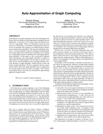
1234567 -FunctionDecl . f ’double (const vector double &)’ -ParmVarDecl . msg ’const vector double &’. ‘-CompoundAssignOperator . ’double’ lvalue ’ ’ ComputeLHSTy ’double’ ComputeResultTy ’double’ -DeclRefExpr . ’double’ lvalue Var 0x104305140 ’sum’ ’double’ . -DeclRefExpr . ’const vector double ’:’const class std::vector double. ’ lvalue ParmVar . ’msg’Figure 3: An AST Example30some of them are not. We can not calibrate all of them. Consider anexample, c is the final answer and c a b. Assume we cancalibrate all three variables a, b and c by multiplying a constant.We may calibrate both a and b, or calibrate only c, which all leadto unbiased result. But calibrating a and c, or all three variablesleads to biased result.f′fdist. (in percentage)error25(a) Iteration Threshold4.2.2 AST and Functions ReplacementSome approximation patterns, like those in Section 4.1.2 and4.1.3, treat the function f (·) as nothing but a black box. For example, for the result memorization in Algo. 1, the synthesized programadds verification condition, and delegates input to f (·) when necessary. An additional storage is used to store the memorized result.The implementation is straightforward, even without the AST.5. SYSTEM CONSIDERATIONSIn this section, beyond straightforward implementation, we introduce several system-dependent issues which help better performance and exploration.5.1Lightweight SamplersIn Source Code 1, Line 4, we propose a simple sampler whichaccesses every five messages. This sampler is ultra-lightweight buti

A classical work-flow of graph computing is shown in Fig. 1(a). A graph algorithm, represented by a UDF, is implemented by the end-user. The end-user passes it to the graph computing system. The system executes it on vertices iteratively, and passes the final result back to the user. End-User Graph Execution Result UDF System Iterative (a .