WIXLIB

3.15A currency graph showing the possible exchanges. Cycles correspond to theprocess of going from one currency to another to another and ultimately endingup with the starting currency.604.1Two graphs that have identical degree sequences, but are not isomorphic.4.2The graph K3 has six automorphisms, one for each element in S3 the setof all permutations on 3 objects. These automorphisms are (i) the identityautomorphism that maps all vertices to themselves; (ii) the automorphism thatexchanges vertex 1 and 2; (iii) the automorphism that exchanges vertex 1 and3; (iv) the automorphism that exchanges vertex 2 and 3; (v) the automorphismthat sends vertex 1 to 2 and 2 to 3 and 3 to 1; and (vi) the automorphism thatsends vertex 1 to 3 and 3 to 2 and 2 to 1.704.3The star graphs S3 and S9 .714.4The adjacency matrix of a graph with n vertices is an n n matrix with a 1at element (i, j) if and only if there is an edge connecting vertex i to vertex j;otherwise element (i, j) is a zero.74664.5Computing the eigenvalues and eigenvectors of a matrix in Matlab can beaccomplished with the eig command. This command will return the eigenvalueswhen used as: d eig(A) and the eigenvalues and eigenvectors when used as[V D] eig(A). The eigenvectors are the columns of the matrix V.784.6Two graphs with the same eigenvalues that are not isomorphic are illustrated.805.1A matrix with 4 vertices and 5 edges. Intuitively, vertices 1 and 4 should havethe same eigenvector centrality score as vertices 2 and 3.875.2A Markov chain is a directed graph to which we assign edge probabilities so thatthe sum of the probabilities of the out-edges at any vertex is always 1.895.3An induced Markov chain is constructed from a graph by replacing every edgewith a pair of directed edges (going in opposite directions) and assigning aprobability equal to the out-degree of each vertex to every edge leaving thatvertex.925.4A set of triangle graphs.955.5A simple social network.985.6A graph partition using positive and negative entries of the Fiedler vector.996.1Feasible Region and Level Curves of the Objective Function: The shaded regionin the plot is the feasible region and represents the intersection of the fiveinequalities constraining the values of x1 and x2 . On the right, we see theoptimal solution is the “last” point in the feasible region that intersects a levelset as we move in the direction of increasing profit.1046.2An example of infinitely many alternative optimal solutions in a linearprogramming problem. The level curves for z(x1 , x2 ) 18x1 6x2 are parallelto one face of the polygon boundary of the feasible region. Moreover, this sidecontains the points of greatest value for z(x1 , x2 ) inside the feasible region. Anyviii

6.36.46.57.17.27.37.47.57.67.77.87.9combination of (x1 , x2 ) on the line 3x1 x2 120 for x1 [16, 35] will providethe largest possible value z(x1 , x2 ) can take in the feasible region S.105Matlab input for solving the diet problem. Note that we are solving aminimization problem. Matlab assumes all problems are mnimization problems,so we don’t need to multiply the objective by 1 like we would if we startedwith a maximization problem.110The Gradient Cone: At optimality, the cost vector c is obtuse with respect tothe directions formed by the binding constraints. It is also contained inside thecone of the gradients of the binding constraints, which we will discuss at lengthlater.112In this problem, it costs a certain amount to ship a commodity along each edgeand each edge has a capacity. The objective is to find an allocation of capacityto each edge so that the total cost of shipping three units of this commodityfrom Vertex 1 to Vertex 4 is minimized.117A cut is defined as follows: in each directed path from v1 to vm , we choose anedge at capacity so that the collection of chosen edges has minimum capacity(and flow). If this set of edges is not an edge cut of the underlying graph, weadd edges that are directed from vm to v1 in a simple path from v1 to vm in theunderlying graph of G.124Two flows with augmenting paths and one with no augmenting paths areillustrated.125The result of augmenting the flows shown in Figure 7.2.126The Edmonds-Karp algorithm iteratively augments flow on a graph until noaugmenting paths can be found. An initial zero-feasible flow is used to start thealgorithm. Notice that the capacity of the minimum cut is equal to the totalflow leaving Vertex 1 and flowing to Vertex 4.127Illustration of the impact of an augmenting path on the flow from v1 to vm .127Games to be played flow from an initial vertex s (playing the role of v1 ). Fromhere, they flow into the actual game events illustrated by vertices (e.g., NY-BOSfor New York vs. Boston). Wins and loses occur and these wins flow across theinfinite capacity edges to team vertices. From here, the games all flow to thefinal vertex t (playing the role of vm ).130Optimal flow was computed using the Edmonds-Karp algorithm. Notice aminimum capacity cut consists of the edges entering t and not all edges leavings are saturated. Detroit cannot make the playoffs.131A maximal matching and a perfect matching. Note no other edges can beadded to the maximal matching and the graph on the left cannot have a perfectmatching.132In general, the cardinality of a maximal matching is not the same as thecardinality of a minimal vertex covering, though the inequality that thecardinality of the maximal matching is at most the cardinality of the minimalcovering does hold.134ix

8.18.28.38.48.59.19.29.39.410.110.210.310.4A graph coloring. We need three colors to color this graph.137At the first step of constructing G , we add three vertices {T, F, B} that form acomplete subgraph.1420At the second step of constructing G , we add two vertices vi and vi to G andan edge {vi , vi0 }142At the third step of constructing G, we add a “gadget” that is built specificallyfor term φj .143When φj evaluates to false, the graph G is not 3-colorable as illustrated insubfigure (a). When φj evaluates to true, the resulting graph is colorable. Bythe label TFT, we mean v(xj1 ) v(xj3 ) TRUE and vj2 FALSE.144 Three random graphs in the same random graph family G 10, 12 . The first twographs, which have 21 edges, have probability 0.52 1 0.52 4. The third graph,which has 24 edges, has probability 0.52 4 0.52 1.148A path graph with 4 vertices has exactly 4!/2 12 isomorphic graphs obtainedby rearranging the order in which the vertices are connected.151There are 4 graphs in the isomorphism class of S3 , one for each possible centerof the star.152The 4 isomorphism types in the random graph family G(5, 3). We show thatthere are 60 graphs isomorphic to this first graph (a) inside G(5, 3), 20 graphsisomorphic to the second graph (b) inside G(5, 3), 10 graphs isomorphic to thethird graph (c) inside G(5, 3) and 30 graphs isomorphic to the fourth graph (d)inside G(5, 3).153The cycle space of a graph can be thought of as all the cycles contained in thatgraph along with the subgraphs consisting of cycles that only share vertices butno edges. This is illustrated in this figure.162A fundamental cycle of a graph G (with respect to a spanning forest F ) is acycle created from adding an edge from the original edge set of G (not in F ) toF.163The cut space of a graph can be thought of as all the minimal cuts contained inthat graph along with the subgraphs consisting of minimal cuts that only sharevertices but no edges. This is illustrated in this figure.164A fundamental edge cut of a graph G (with respect to a spanning forest F ) is apartition cut created from partitioning the vertices based on a cut in a spanningtree and then constructing the resulting partition cut.165x

PrefaceThis is version two of set of lecture notes for Math 485–Penn State’s undergraduate GraphTheory course. Since I use these notes while I teach, there (still) may be typographical errorsthat I noticed in class, but did not fix in the notes. If you see a typo, send me an e-mail andI’ll add an acknowledgement.The lecture notes are loosely based on Gross and Yellen’s Graph Theory and It’s Applications [GY05], Bollobás’ Modern Graph Theory [Bol00], Diestel’s Graph Theory, Wolseyand Nemhauser’s Integer and Combinatorial Optimization [Die10], Korte and Vygen’s Combinatorial Optimization [KV08] and several other books that are cited in these notes. Allof the books mentioned are good books (some great) but I like different parts of each ofthem. Consequently I’ve combined the material in a format for that can be used easily inan undergraduate mathematics class. Many of the proofs in this set of notes are adaptedfrom the textbooks with some minor additions. One thing that is included in these notesis a treatment of max flow theorems from the perspective linear optimization. This is notcovered in most graph theory books, while graph theoretic principles are not covered in manylinear or combinatorial optimization books. I should note, Bondy and Murty discuss LinearProgramming in their book Graph Theory. The best book on the topic of combinatorialoptimization is by far Korte and Vygen’s, who do cover linear programming in their latest edition. There is also a heavy emphasis on algebraic graph theory because I like linearalgebra and this is one of the most useful parts of graph theory.In order to use these notes successfully, you should have taken a course in combinatorialproof (Math 311W at Penn State) and ideally matrix algebra (Math 220 at Penn State),though courses in Linear Programming (Math 484 at Penn State) wouldn’t hurt. I reviewa substantial amount of the material you will need, but it’s always good to have coveredprerequisites before you get to a class. That being said, I hope you enjoy using these notes!xi

CHAPTER 1Introduction to Graph Theory1. An Overview of Graph TheoryGraph Theory began with Leonhard Euler in his study of the Bridges of Königsburgproblem. Here’s how it started: The city of Königsburg exists as a collection of islandsconnected by bridges as shown in Figure 1.1. The problem Euler wanted to analyze was: IsIslandsBridgeCADBFigure 1.1. The city of Königsburg is built on a river and consists of four islands,which can be reached by means of seven bridges. The question Euler was interestedin answering is: Is it possible to go from island to island traversing each bridgeonly once? (Picture courtesy of Wikipedia and Wikimedia Commons: http://en.wikipedia.org/wiki/File:Konigsberg bridges.png)it possible to go from island to island traversing each bridge only once? This was assumingthat there was no trickery such as using a boat. Euler analyzed the problem by simplifyingthe representation and as a result created modern graph theory. We’ll come back to Euler’ssolution later.Since Euler solved this very first problem in Graph Theory, the field has exploded, becoming one of the most important areas of applied mathematics we currently study. Generallyspeaking, Graph Theory is a branch of Combinatorics but it is closely connected to AppliedMathematics, Optimization Theory and Computer Science. At Penn State (for example)if you want to start a bar fight between Math and Computer Science (and possibly Electrical Engineering) you might claim that Graph Theory belongs (rightfully) in the MathDepartment. (This is only funny because there is a strong group of graph theorists inour Computer Science Department.) In reality, Graph Theory is cross-disciplinary betweenMath, Computer Science, Electrical Engineering and Operations Research1. Here are someof the subjects within Graph Theory that are of interest to people in these disciplines:1Seemy note on Network Science below.1

(1) Optimization Problems on Graphs: Problems of optimization on graphs generallytreat a graph structure like a road network and attempt to maximize flow along thatnetwork while minimizing costs. There are many classical optimization problemsassociated to graphs and this field is sometimes considered a sub-discipline withinCombinatorial Optimization.(2) Topological Graph Theory: Asks questions about methods of embedding graphs intotopological spaces (like R2 or on the surface of a torus) so that certain properties aremaintained. For example, the question of planarity asks: Can a graph be drawn onthe plane in such a way so that no two edge cross. Clearly, the bridges of Königsburggraph had that property, but not all graphs do.(3) Graph Coloring: A question related both to optimization and to planarity asks howmany colors does it take to color each vertex (or edge) of a graph so that no twoadjacent vertices have the same color. Attempting to obtain a coloring of a graphhas several applications to scheduling and computer science.(4) Analytic Graph Theory: Is the study of randomness and probability applied tographs. Random graph theory is a subset of this study. In it, we assume that agraph is drawn from a probability distribution that returns graphs and we studythe properties that certain distributions of graphs have.(5) Algebraic Graph Theory: Is the application of abstract algebra (sometimes associated with matrix groups) to graph theory. Many interesting results can be provedabout graphs when using matrices and other algebraic properties.Obviously this is not a complete list of all the various problems and applications of GraphTheory. However, this is a list of some of the things we may touch on in the class. Thetextbook [GY05] is a good place to start on some of these topics. Another good sourceis [BM08], which I used for some of these notes. [Bol01] and [Bol00] are classics by oneof the absolute masters of the field Bollobás and Diestel’s [Die10] book is a pleasant read(it actually used to be much shorter). For the combinatorial optimization element of graphtheory, turn to Nemhauser and Wolsey [WN99] as well as the second part of Bazarra etal.’s Linear Programming and Network Flows [BJS04]. Another reasonable book is [PS98],though it’s a bit older, it’s much less expensive than the others. In that same theme,[Tru94] and [Cha84] are also inexpensive little introductions to Graph Theory that are notas comprehensive as Gross and Yellen or Bondy and Murty, but they are nice to have inone’s library for easier reading. In particular, [Cha84] spends a lot of time on applicationsrather than theory.2. Graphs, Multi-Graphs, Simple GraphsDefinition 1.1 (Graph). A graph is a tuple G (V, E) where V is a (finite) set ofvertices and E is a finite collection of edges. The set E contains elements from the unionof the one and two element subsets of V . That is, each edge is either a one or two elementsubset of V .Definition 1.2 (Self-Loop). If G (V, E) is a graph and v V and e {v}, thenedge e is called a self-loop. That is, any edge that is a single element subset of V is called aself-loop.2

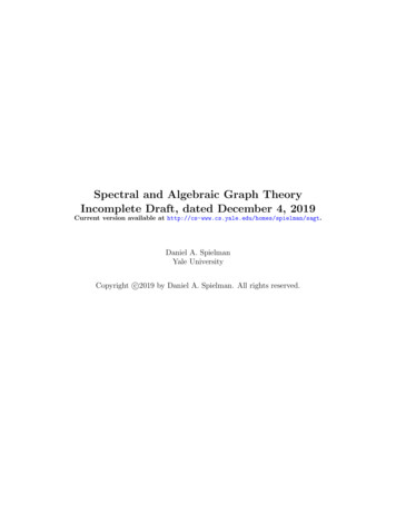
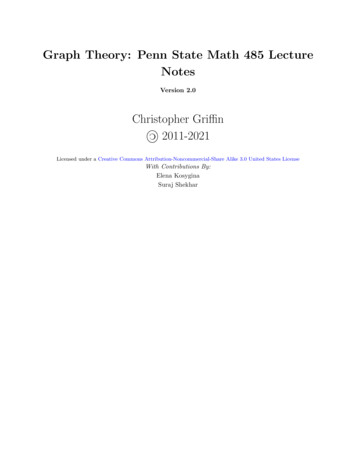
Definition 1.3 (Vertex Adjacency). Let G (V, E) be a graph. Two vertices v1 andv2 are said to be adjacent if there exists an edge e E so that e {v1 , v2 }. A vertex v isself-adjacent if e {v} is an element of E.Definition 1.4 (Edge Adjacency). Let G (V, E) be a graph. Two edges e1 and e2 aresaid to be adjacent if there exists a vertex v so that v is an element of both e1 and e2 (assets). An edge e is said to be adjacent to a vertex v if v is an element of e as a set.Definition 1.5 (Neighborhood). Let G (V, E) be a graph and let v V . Theneighbors of v are the set of vertices that are adjacent to v. Formally:(1.1)N (v) {u V : e E (e {u, v} or u v and e {v})}In some texts, N (v) is called the open neighborhood of v while N [v] N (v) {v} is calledthe closed neighborhood of v. This notation is somewhat rare in practice. When v is anelement of more than one graph, we write NG (v) as the neighborhood of v in graph G.Remark 1.6. Expression 1.1 is readN (v) is the set of vertices u in (the set) V such that there exists an edge ein (the set) E so that e {u, v} or u v and e {v}.The logical expression x (R(x)) is always read in this way; that is, there exists x so thatsome statement R(x) holds. Similarly, the logical expression y (R(y)) is read:For all y the statement R(y) holds.Admittedly this sort of thing is very pedantic, but logical notation can help immensely insimplifying complex mathematical expressions2.Remark 1.7. The difference between the open and closed neighborhood of a vertex canget a bit odd when you have a graph with self-loops. Since this is a highly specialized case,usually the author (of the paper, book etc.) will specify a behavior.Example 1.8. Consider the set of vertices V {1, 2, 3, 4}. The set of edgesE {{1, 2}, {2, 3}, {3, 4}, {4, 1}}Then the graph G (V, E) has four vertices and four edges. It is usually easier to representthis graphically. See Figure 1.2 for the visual representation of G. These visualizationsare constructed by representing each vertex as a point (or square, circle, triangle etc.) andeach edge as a line connecting the vertex representations that make up the edge. That is, letv1 , v2 V . Then there is a line connecting the points for v1 and v2 if and only if {v1 , v2 } E.In this example, the neighborhood of Vertex 1 is Vertices 2 and 4 and Vertex 1 is adjacentto these vertices.2WhenI was in graduate school, I always found Real Analysis to be somewhat mysterious until I gotused to all the ’s and δ’s. Then I took a bunch of logic courses and learned to manipulate complex logicalexpressions, how they were classified and how mathematics could be built up out of Set Theory. Suddenly,Real Analysis (as I understood it) became very easy. It was all about manipulating logical sentences aboutthose ’s and δ’s and determining when certain logical statements were equivalent. The moral of the story:if you want to learn mathematics, take a course or two in logic.3

1243Figure 1.2. It is easier for explanation to represent a graph by a diagram in whichvertices are represented by points (or squares, circles, triangles etc.) and edges arerepresented by lines connecting vertices.Definition 1.9 (Degree). Let G (V, E) be a graph and let v V . The degree of v,written deg(v) is the number of non-self-loop edges adjacent to v plus two times the numberof self-loops defined at v. More formally:deg(v) {e E : u V (e {u, v})} 2 {e E : e {v}} Here if S is a set, then S is the cardinality of that set.Remark 1.10. Note that each vertex in the graph in Figure 1.2 has degree 2.Example 1.11. If we replace the edge set in Example 1.8 with:E {{1, 2}, {2, 3}, {3, 4}, {4, 1}, {1}}then the visual representation of the graph includes a loop that starts and ends at Vertex 1.This is illustrated in Figure 1.3. In this example the degree of Vertex 1 is now 4. We obtainSelf-Loop1243Figure 1.3. A self-loop is an edge in a graph G that contains exactly one vertex.That is, an edge that is a one element subset of the vertex set. Self-loops areillustrated by loops at the vertex in question.this by counting the number of non self-loop edges adjacent to Vertex 1 (there are 2) andadding two times the number of self-loops at Vertex 1 (there is 1) to obtain 2 2 1 4.Example 1.12. Recall the problem of the Königsburg bridges (see Figure 1.1). LikeEuler, we want to answer the question: Is it possible to go from island to island traversingeach bridge only once? We construct a graph to analyze the problem. Assume that we treateach island as a vertex and each bridge as an egde. The resulting graph is illustrated inFigure 1.4.4

Island(s)CADBridgeBFigure 1.4. Representing each island as a dot and each bridge as a line or curveconnecting the dots simplifies the visual representation of the seven KönigsburgBridges.Note this representation dramatically simplifies the analysis of the problem in so far aswe can now focus only on

Chapter 1. Introduction to Graph Theory1 1. An Overview of Graph Theory1 2. Graphs, Multi-Graphs, Simple Graphs2 3. Directed Graphs7 4. Elementary Graph Properties: Degrees and Degree Sequences9 5. Subgraphs14 6. Graph Complement, Cliques and Independent Sets15 Chapter 2. More De nitions and Theorems19 1. Paths, Walks, and Cycles19 2.