WIXLIB

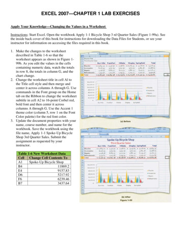
EXCEL 2007—CHAPTER 1 LAB EXERCISESApply Your Knowledge—Changing the Values in a WorksheetInstructions: Start Excel. Open the workbook Apply 1-1 Bicycle Shop 3 rd Quarter Sales (Figure 1-99a). Seethe inside back cover of this book for instructions for downloading the Data Files for Students, or see yourinstructor for information on accessing the files required in this book.1. Make the changes to the worksheetdescribed in Table 1-6 so that theworksheet appears as shown in Figure 199b. As you edit the values in the cellscontaining numeric data, watch the totalsin row 8, the totals in column G, and thechart change.2. Change the worksheet title in cell Al tothe Title cell style and then merge andcenter it across columns A through G. Usecommands in the Font group on the Hometab on the Ribbon to change the worksheetsubtitle in cell A2 to 16-point Corbel red,bold font and then center it acrosscolumns A through G. Use the Accent 1theme color (column 5, row 1 on the FontColor palette) for the red font color.3. Update the document properties with yourname, course number, and name for theworkbook. Save the workbook using thefile name, Apply 1-1 Spoke-Up BicycleShop 3rd Quarter Sales. Submit theassignment as requested by yourinstructor.Table 1-6 New Worksheet DataCell Change Cell Contents ToA1Spoke-Up Bicycle ShopB411869.2E49157.83D65217.92F66239.46B73437.64

Extend Your Knowledge—Formatting Cells and Inserting Multiple ChartsInstructions: Start Excel. Open the workbook Extend 1-1 Pack-n-Away Shipping. See the inside back cover ofthis book for instructions for downloading the Data Files for Students, or see your instructor for information onaccessing the files required in this book. Perform the following tasks to format cells in the worksheet and to addtwo charts to the worksheet.1. Use the commands in the Fontgroup on the Home tab on theRibbon to change the font of thetitle in cell Al to 24-point Arial,red, bold and subtitle of theworksheet to 16-point ArialNarrow, blue, bold.2. Select the range A3:E8, click theInsert tab on the Ribbon and thenclick the Dialog Box Launcher inthe Charts group on the Ribbonto open the Insert Chart dialogbox (Figure 1-100).3. Insert a Stacked Line chart byclicking the Stacked Line chartin the gallery and then clickingthe OK button. Move the charteither below or to the right of thedata in the worksheet. Click theDesign tab and apply a chartstyle to the chart.4. If necessary, reselect the rangeA3:E8 and follow Step 3 aboveto insert a 3-D Area chart in theworksheet. You may need to use the scroll box on the right side of the Insert Chart dialog box to view theArea charts in the gallery. Move the chart either below or to the right of the data so that each chart does notoverlap the Stacked Line chart. Choose a different chart style for this chart than the one you selected for theStacked Line chart.5. Resize each chart so that each snaps to the worksheet gridlines. Make certain that both charts are visiblewith the worksheet data without the need to scroll the worksheet.6. Update the document properties with your name, course number, and name for the workbook.7. Save the workbook using the file name, Extend 1-1 Pack-n-Away Shipping Charts. Submit the assignmentas requested by your instructor.

Make It Right—Correcting Formatting and Values in a WorksheetInstructions: Start Excel. Open the workbook Make It Right 1-1 Book Sales. See the inside back cover of thisbook for instructions for downloading the Data Files for Students, or see your instructor for information onaccessing the files required for this book. Correct the following formatting problems and data errors (Figure 1101) in the worksheet, while keeping in mind the guidelines presented in this chapter.1. Merge and center theworksheet title andsubtitle appropriately.2. Format the worksheettitle with a cell styleappropriate for aworksheet title.3. Format the subtitleusing commands in theFont group on theRibbon.4. Correct the spellingmistake in cell Al bychanging Bool toBooks.5. Apply properformatting to thecolumn headers andtotal row.6. Adjust column sizes sothat all data in eachcolumn is visible.7. Use the SUM function to create the grand total for annual sales.8. The SUM function in cell E9 does not sum all of the numbers in the column. Correct this error by editingthe range for the SUM function in the cell.9. Resize and move the chart so that it is below the worksheet data and does not extend past the right edge ofthe worksheet data. Be certain to snap the chart to the worksheet gridlines by holding down the ALT key asyou resize the chart.10. Update the document properties with your name, course number, and name for the workbook. Save theworkbook using the file name, Make It Right 1-1 Eric's Used Books Annual Sales. Submit the assignment asrequested by your instructor.

Lab 1: Annual Cost of Goods WorksheetProblem: You work part-time as a spreadsheet specialist for Kona's Expresso Coffee, one of the up-and-comingcoffee franchises in the United States. Your manager has asked you to develop an annual cost of goods analysisworksheet similar to the one shown in Figure 1-102.Instructions: Perform the following tasks.1. Start Excel. Enter the worksheet title, Kona's Expresso Coffee, in cell A1 and the worksheet subtitle, AnnualCost of Goods, in cell A2. Beginning in row 3, enter the store locations, costs of goods, and suppliescategories shown in Table 1-7.2. Use the SUM function to determine the totals for each store location, type of supply, and company grandtotal.3. Use Cell Stylesin the Stylesgroup on theHome tab onthe Ribbon toformat theworksheet titlewith the Titlecell style.Center the titleacross columnsA through G.Do not beconcerned if theedges of theworksheet titleare notdisplayed.4. Use buttons inthe Font groupon the Home tab on the Ribbon to format the worksheet subtitle to 14-point Calibri dark blue, bold font andcenter it across columns A through G.5. Use Cell Styles in the Styles group on the Home tab on the Ribbon to format the range A3:G3 with theHeading 2 cell style, the range A4:G7 with the 20% - Accent1 cell style, and the range A8:G8 with the Totalcell style. Use the buttons in the Number group on the Home tab on the Ribbon to apply the AccountingNumber format to the range B4:G4 and the range B8:G8. Use the buttons in the Number group on the Hometab on the Ribbon to apply the Comma Style to the range B5:G7. Adjust any column widths to the widesttext entry in each column.

6. Select the range A3:F7 and then insert a 3-D Clustered Column chart. Apply the Style 5 chart style to thechart. Move and resize the chart so that it appears in the range A10:G22. If the labels along the horizontalaxis (x-axis) do not appear as shown in Figure 1-102, then drag the right side of the chart so that it isdisplayed in the range A10:G22.7. Update the document properties with your name, course number, and name for the workbook.8. Save the workbook using the file name Lab 1-1 Konas Expresso Coffee Annual Cost of Goods.9. Print the worksheet.10. Make the following two corrections to the sales amounts: 9,648.12 for Seattle Condiments (cell E6), 12,844.79 for Chicago Pastries (cell C7). After you enter the corrections, the company totals in cell G8should equal 462,135.04.11. Print the revised worksheet. Close the workbook without saving the changes. Submit the assignment asrequested by your instructor.Lab 2: Annual Sales Analysis WorksheetProblem: As the chief accountant for Scissors Office Supply, Inc., you have been asked by the sales manager tocreate a worksheet to analyze the annual sales for the company by location and customer type category (Figure1-103). The office locations and corresponding sales by customer type for the year are shown in Table 1-8.Instructions: Perform the following tasks.1. Create the worksheet shown in Figure 1-103 using the data in Table 1-8.2. Use the SUM function to determine totals sales for the four offices, the totals for each customer type, andthe company total. Add column and row headings for the totals row and totals column, as appropriate.3. Format the worksheet title with the Title cell style and center it across columns A through F. Use the Fontgroup 0It the Ribbon to format the worksheet subtitle to 16-point Cambria green, and bold font. Center thetitle across columns A through F.4. Format the range A3:F3 with the Heading 2 cell style, the range A4:F8 with the 20% - Accent35. cell style, and the range A9:F9 with the Total cell style. Use the Number group on the Ribbon to formatcells B4:F4 and B9:F9 with the Accounting Number Format and cells B5:F8 with the Comma Style numericformat. Adjust the width of column A in order to fit contents of the column.6. Chart the range A3:E8. Insert a 100% Stacked Column chart for the range A3:E8, as shown in Figure 1-103,by using the Column button on the Insert tab on the Ribbon. Use the chart location A11:F22.7. Update the document properties 'with your name, course number, and name for the workbook.8. Save the workbook using the file name, Lab 1-2 Scissors Office Supply Annual Sales. Print the worksheet.9. Two corrections to the figures were sent in from the accounting department. The correct sales are 98,342.16 for Miami's annual Small Business sales (cell C5) and 48,933.75 for10. St. Louis's annual Nonprofit sales (cell D8). After you enter the two corrections, the company total in cellF9 should equal 2,809,167.57. Print the revised worksheet.11. Use the Undo button to change the worksheet back to the original numbers in Table 1-8. Use12. the Redo button to change the worksheet back to the revised state.13. Close Excel without saving the latest changes. Start Excel and open the workbook saved in

14. Step 7. Double-click cell E6 and use in-cell editing to change the Santa Fe annual Large Business sales (cellE6) to 154,108.49. Write the company total in cell F9 at the top of the first printout. Click the Undo button.15. Click cell Al and then click the Merge & Center button to split cell A1 into cells A1, B1,16. C1, D1, E1, and F1. To merge the cells into one again, select the range A1:F1 and then click the Merge &Center button on the Home tab on the Ribbon.17. Close the workbook without saving the changes. Submit the assignment as requested by your instructor.Lab 3: College Cost and Financial Support WorksheetProblem: Attending college is an expensive proposition and your resources are limited. To plan for your fouryear college career, you have decided to organize your anticipated resources and costs in a worksheet. The datarequired to prepare your worksheet is shown in Table 1-9.