Transcription
Learning Feature Representations with K-meansAdam Coates and Andrew Y. NgStanford University, Stanford CA 94306, USA{acoates,ang}@cs.stanford.eduOriginally published in: G. Montavon, G. B. Orr, K.-R. Müller (Eds.), NeuralNetworks: Tricks of the Trade, 2nd edn, Springer LNCS 7700, 2012.Abstract. Many algorithms are available to learn deep hierarchies offeatures from unlabeled data, especially images. In many cases, thesealgorithms involve multi-layered networks of features (e.g., neural networks) that are sometimes tricky to train and tune and are difficult toscale up to many machines effectively. Recently, it has been found thatK-means clustering can be used as a fast alternative training method.The main advantage of this approach is that it is very fast and easilyimplemented at large scale. On the other hand, employing this methodin practice is not completely trivial: K-means has several limitations, andcare must be taken to combine the right ingredients to get the systemto work well. This chapter will summarize recent results and technicaltricks that are needed to make effective use of K-means clustering forlearning large-scale representations of images. We will also connect theseresults to other well-known algorithms to make clear when K-means canbe most useful and convey intuitions about its behavior that are usefulfor debugging and engineering new systems.1IntroductionA major goal in machine learning is to learn deep hierarchies of features for othertasks. For instance, given a set of unlabeled images, many current algorithmsseek to greedily learn successive layers of features that will make subsequentclassification tasks (e.g., object recognition) easier to accomplish. A typical approach taken in the literature is to use an unsupervised learning algorithm totrain a model of the unlabeled data and then use the results to extract interesting features from the data [35,21,31]. Depending on the choice of unsupervisedlearning scheme, it is sometimes difficult to make these systems work well. Therecan be many hyper-parameters and not much intuition for how to tune them.More recently, we have found that using K-means clustering as the unsupervisedlearning module in these types of “feature learning” pipelines can lead to excellent results, often rivaling state-of-the-art systems [11]. In this chapter, we willreview some of this work with added notes on useful tricks and observations thatare helpful for building large-scale feature learning systems.K-means has already been identified as a successful method to learn features from images by computer vision researchers. The popular “bag of features”
model [13,28] from the computer vision community is very similar to the pipelinethat we will use in this chapter, and many conclusions here are similar to thoseidentified by vision researchers [18,1]. In this chapter, however, we will focus onthe ingredients needed to make K-means work well in a setting similar to thatused by other deep learning and feature learning systems: learning directly fromraw inputs (pixel intensities) and building multi-layered hierarchies, as well asconnecting K-means to other well-known feature learning systems.The classic K-means clustering algorithm finds cluster centroids that minimize the distance between data points and the nearest centroid. Also called“vector quantization”, K-means can be viewed as a way of constructing a “dictionary” D Rn k of k vectors so that a data vector x(i) Rn , i 1, . . . , mcan be mapped to a code vector that minimizes the error in reconstruction.In this chapter, we will use a modified version of K-means (sometimes called“gain shape” vector quantization [41], or “spherical K-means” [14]) that finds Daccording to:Xminimize Ds(i) x(i) 22D,sisubject to s(i) 0 1, iand D(j) 2 1, jwhere s(i) is a “code vector” associated with the input x(i) , and D(j) is the j’thcolumn of the dictionary D. The goal here is to find a dictionary D and a newrepresentation, s(i) , of each example x(i) that satisfies several criteria. First, givens(i) and D, we should be able to reconstruct the original x(i) well; in particular,we aim to minimize the squared difference between x(i) and its correspondingreconstruction Ds(i) . This goal is optimized under two constraints. The firstconstraint, s(i) 0 1, means that each s(i) is constrained to have at most onenon-zero entry. Thus we are searching not only for a new representation of x(i)that preserves it as well as possible, but also for a very simple or parsimoniousrepresentation. The second constraint requires that each dictionary column haveunit length, preventing them from becoming arbitrarily large or small. Otherwise(i)we could arbitrarily rescale D(j) and the corresponding sj without effect.This algorithm is very similar in spirit to other algorithms for learning efficient coding schemes, such as sparse coding [34,17]:minimizeD,sX Ds(i) x(i) 22 λ s(i) 1isubject to D(j) 2 1, j.Sparse coding optimizes the same type of reconstruction objective, but constrainsthe complexity of s(i) by adding a penalty λ s(i) 1 that encourages s(i) to besparse. This is similar to the constraint used by K-means ( s(i) 0 1), butallows more than one non-zero entry in each s(i) , enabling a much more accuraterepresentation of each x(i) while still requiring each s(i) to be simple.
From their descriptions above, it is no surprise that K-means and more sophisticated dictionary-learning schemes like sparse coding are often interchangeable—differing in their optimization objectives, but producing code vectors s(i) anddictionaries D that accomplish similar goals. Empirically though, sparse codingappears to be a better performer in many applications. For instance, replacingK-means with sparse coding in the classic bag-of-features model has been shownto significantly improve image recognition results [39]. Despite its simplicity,however, K-means is still a very useful algorithm for learning features due to itsspeed and scalability. Sparse coding requires us to solve a convex optimizationproblem [36,15,32] for every s(i) repeatedly during the learning procedure andthus is very expensive to deploy at large scale. For K-means, by contrast, theoptimal s(i) used in the algorithm above is simply:(i)sj D(j) x(i)if j arg max D(l) x(i) 0otherwise.l(1)Because this can be done very quickly (and solving for D given s is also easy), wecan train very large dictionaries rapidly by alternating optimization of D and s.As well, K-means does not have any parameters requiring tuning other than k,the number of centroids, making it relatively easy to get working. The surpriseis that large dictionaries learned by K-means often work very well in practiceprovided we mix in a few other ingredients that are less commonly documentedin other works. This chapter is about what these ingredients are as well as someintuition about why they are needed and how they affect results. For most ofthis work, we will use images (or image patches) as input data to the algorithm,but the basic principles are applicable to other types of data as well.2Data, Pre-processing and InitializationWe will begin with a dataset composed of small image patches. For concreteness,we will work with 16-by-16 pixel grayscale patches represented as a vector of 256pixel intensities (i.e., x(i) R256 ), but color patches can also be used similarly.These patches can be collected from unlabeled imagery by cropping out random16-by-16 chunks. In order to build a “complete” dictionary (i.e., a dictionarywith at least 256 centroids), we should ensure that there will be enough patchesso that each cluster can claim a reasonable number of inputs. For 16-by-16 graypatches, m 100, 000 patches is enough. In practice, we will often need moredata to train a K-means dictionary than is necessary for other algorithms (e.g.,sparse coding), since each data point contributes to just 1 centroid in the end.Usually the added expense is easily offset by the speed of training. For notationalconvenience, we will assume that our data points are packed into the columns ofa matrix X Rn m . (Similarly, we will denote by S the matrix whose columnsare the code vectors s(i) from Eq. (1).)
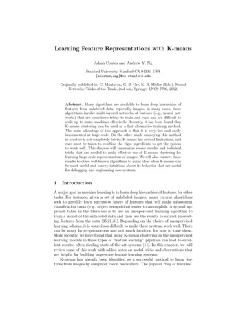
2.1Pre-processingBefore running a learning algorithm on our input data points x(i) , it is useful tonormalize the brightness and contrast of the patches. That is, for each x(i) wesubtract out the mean of the intensities and divide by the standard deviation. Asmall value is added to the variance before division to avoid divide by zero andalso suppress noise. For pixel intensities in the range [0, 255], adding 10 to thevariance is often a good starting point:x̃(i) mean(x̃(i) )x(i) pvar(x̃(i) ) 10where x̃(i) are unnormalized patches and “mean” and “var” are the mean andvariance of the elements of x̃(i) .(a)(b)(c)Fig. 1: (a) Centroids learned by K-means from natural images without whitening.(b) A cartoon depicting the effect of whitening on the K-means solution. Left:unwhitened data, where the centroids tend to be biased by the correlated data.Right: whitened data, where centroids are more orthogonal. (c) Centroids learnedfrom whitened image patches.After normalization, we can try to run K-means on the new input patches.The centroids that are obtained (i.e., the columns of the dictionary D) are visualized as patches in Figure 1a. It can be seen that K-means tends to learnlow-frequency edge-like centroids. This result has been reproduced many timesin the past [16,37,2]. Unfortunately, it turns out that these centroids tend towork poorly in recognition tasks [11]. One explanation for this result is that thecorrelations between nearby pixels (i.e., low-frequency variations in the images)tend to be very strong even after brightness and contrast normalization. In thepresence of these correlations, K-means tends to generate many highly correlatedcentroids rather than spreading the centroids out to span the data more evenly.A cartoon depicting this problem is shown on the left of Figure 1b. To remedythis situation, one should use whitening (also called “sphering”) to rescale theinput data to remove these correlations [22]. This tends to cause K-means to
allocate more centroids in the orthogonal directions, as shown on the right ofFigure 1b.A simple choice of whitening transform is the ZCA whitening transform. IfV DV cov(x) is the eigenvalue decomposition of the covariance of the datapoints x, then the whitened points are computed as V (D zca I) 1/2 V x, where zca is a small constant. For contrast-normalized data, setting zca to 0.01 for16-by-16 pixel patches, or 0.1 for 8-by-8 pixel patches is a good starting point.Note that setting this number too small can cause high-frequency noise to beamplified and make learning more difficult. Since rotating the data does not alterthe behavior of K-means, one can also use other whitening transforms such asPCA whitening (which differ from ZCA only by a rotation).Running K-means on whitened image patches yields sharper edge featuressimilar to those discovered by sparse coding, ICA, and others as seen in Figure 1c. This procedure of normalization, whitening, and K-means clustering isan effective “off the shelf” unsupervised learning module that can serve in manyfeature-learning roles. From this point forward, we will assume that whenever weapply K-means to new data that they are normalized and whitened as describedhere. But keep in mind that proper choices of the parameters for normalizationand whitening can sometimes require adjustment for new data sources. Thoughthese are likely best set by cross validation, they can often be tuned visually(e.g., to yield image patches with high contrast, not too much noise, and not toomuch low-frequency undulation).2.2InitializationThe usual K-means clustering algorithm is known to require a number of smalltweaks to avoid common problems like empty clusters. One important consideration is the initialization of the centroids. Though it is common to initializeK-means to randomly-chosen examples drawn from the data, this has been foundto be a poor choice. It is possible that images tend to group too densely in someareas, and thus initializing K-means with randomly chosen patches leads to alarge number of centroids starting close together. Many of these centroids ultimately end up becoming near-empty clusters, as a single cluster accumulatesall of the data points located within a dense area. Instead, it is better to randomly initialize the centroids from a Normal distribution and then normalizethem to unit length. Note that because of the whitening stage, we expect thatthe important components of our data have already been rescaled to a more orless spherical distribution, so initializing to random vectors on a sphere is not aterrible starting point.Other well-known heuristics for improving the behavior of K-means can beuseful. For instance, heuristics for reinitializing empty clusters are commonlyused in other implementations. In practice, the initialization scheme above worksrelatively well for image data. When empty clusters do occur, reinitializing thecentroids with random examples is usually sufficient, but this is rarely neces-
sary.1 In fact, for a sufficiently scalable implementation, we can often train manycentroids and simply throw away clusters that have too few data points.Another minor tweak that improves behavior is to use damped updates ofthe centroids. Specifically, at each iteration we compute new centroids accordingto:Dnew : arg min DS X 22 D Dold 22D (SS I) 1 (XS Dold ) XS DoldDnew : normalize(Dnew ).Note that this form of damping does not affect “big” clusters very much (the(j)j’th column of XS will be large compared to Dold ) and only serves to preventsmall clusters from being pulled too far in a single iteration.Including the initialization and pre-processing, the full K-means training routine presented above is summarized here:1. Normalize inputs:x(i) mean(x(i) )x(i) : p, ivar(x(i) ) norm2. Whiten inputs:[V, D] : eig(cov(x)); // So V DV cov(x)x(i) : V (D zca I) 1/2 V x(i) , i3. Loop until convergence (typically 10 iterations is enough): D(j) x(i) if j arg max D(l) x(i) (i)lsj : j, i 0otherwise.D : XS DD(j) : D(j) / D(j) 2 j1Often, a large number of empty clusters indicates that the whitening or normalizationparameters are improperly tuned, or the data is too high-dimensional for K-meansto be successful.
Fig. 2: The result of running spherical K-means on points sampled from a heavytailed distribution. The K-means “centroids” tend to point in the directions ofthe tails.3Comparison to Sparse Feature LearningAs was shown above, K-means learns oriented edge-like features when applied tonatural images, much like ICA [23] or sparse coding [34]. An important practicalquestion is whether this is accidental (e.g., because edges are so common thatlearning “exemplars” from images is enough to find them) or whether this impliesthat K-means can perform a type of sparse decomposition similar to ICA. Whenwe attempt to apply K-means to other types of data such as audio or featurescomputed by lower layers in a deep network, it is important to understand towhat extent this clustering algorithm mimics well-known projection methods likeICA and what the limitations are. It is clear that because each s(i) is allowed tocontain only a single non-zero entry, K-means tries to learn centroids that singlehandedly explain an entire input image. It is thus not guaranteed that the learnedcentroids will always be like the filters produced by sparse coding or ICA. Thesealgorithms learn genuine “distributed” representations where a single image canbe explained jointly by multiple columns of the dictionary instead of just one.Nevertheless, empirically it turns out that K-means does tend to discover sparseprojections of the data under the right conditions. Because of this property, wecan often use the learned dictionary in a manner similar to the dictionaries orfilters learned by other algorithms that explicitly search for sparse, distributedrepresentations.One intuition for why this tends to occur can be seen in a simple lowdimensional example. Consider the case where our data is sampled from twoindependent, heavy-tailed (sparse) random variables. After normalization, thedata will be most dense near the coordinate axes, and less dense in the quadrants between them. As a result, while K-means will tend to represent manypoints very badly, training 2 centroids on this distribution will tend to yield a
Fig. 3: Top: Three different sparse distributions of images. Bottom: Filters (centroids) identified by K-means with a complete (256-centroid) dictionary.dictionary of basis vectors pointing in the direction of the tails (i.e., in the sparsedirections). This result is illustrated in Figure 2.If the data dimensionality is not too high (e.g., a hundred or so) this “tailseeking” phenomenon also shows up in more complicated scenarios. Figure 3shows examples of three sets of images generated from sparse sources. On theleft (at top), are 16-by-16 images with pixels sampled from independent Laplacedistributions (sparse pixel intensities). In the middle (top) are images composedof a sparse combination of gratings and at right (top) a sparse combination ofnon-orthogonal gabor filters. The bottom row shows the result of learning 256centroids with K-means from 500000 examples drawn from each distribution.It can be seen that K-means does, in fact, roughly recover the sparse projections we would expect. A similar experiment appears in [34] to demonstrate thesource-separation ability of sparse coding—yet K-means tends to recover thesame filters even though these filters are clearly not especially similar to individual images. That is, K-means can potentially do more than merely recover“exemplar” images from the input distribution.When applied to natural images, it is evident that the learned centroids D(j)(as in Figure 1c) are relatively sparse projections of the data. Figure 4a showsa histogram of responses resulting from projecting randomly chosen (whitened)image patches onto 4 different filters. The 4 filters used are: (i) a centroid learnedby K-means, (ii) a basis vector trained via sparse coding, (iii) a randomly selectedimage patch, and (iv) a randomly initialized filter. In the figure, it can be seenthat using the K-means-trained centroid as a linear filter gives us a very sparseprojection of the data. Thus, it appears that relative to other simple choicesK-means does tend to seek out very sparse projections of the data, even thoughits formulation as a clustering algorithm does not aim to do this explicitly.Despite this empirical similarity to ICA and sparse coding, K-means doeshave a major drawback: it turns out that its ability to discover sparse directionsin the data depends heavily on the dimensionality of the input and the quantityof data. In particular, as the dimensionality increases, we need increasingly large
(a)(b)Fig. 4: (a) A comparison of the distribution of linear filter responses when filtersobtained by 4 different methods are applied to natural image patches. K-meanstends to learn filters with very sparse response characteristics similar to sparsecoding—much more sparse than randomly chosen patches or randomly initializedfilters. (b) “Centroids” learned from 64-by-64 pixel patches. At this scale, Kmeans becomes difficult to apply as many clusters become empty or singletons.quantities of data to get clean results. For instance, to obtain the results abovewe had to use a very large number of examples. We can obtain similar resultseasily with sparse coding with just 10000 examples. For very large patches, wemust use even more. Figure 4b shows the results of running K-means on 50000064-by-64 patches—note that while we can capture a few edges, most of theclusters are composed of a single patch from the dataset. At this scale, empty ornear-empty clusters become far more common and extremely large amounts ofdata are needed to make K-means work well. This tradeoff is the main driver indeciding when and how to employ K-means: depending on the dimensionality ofthe input, a certain amount of data will be required (typically much more than isneeded for similar results from sparse coding). For modest dimensionalities (e.g.,hundreds of inputs), this tradeoff can be advantageous because the additionaldata requirements do not outweigh the very large constant-factor speedup thatis gained by training with K-means. For very high dimensionalities, however, itmay well be the case that another algorithm like sparse coding works better oreven faster.4Application to Image RecognitionThe above discussion has provided the basic ingredients needed to turn K-meansinto a simple feature learning method. Given a batch of unlabeled data, we cannow learn a dictionary D whose columns yield more or less sparse projections
of the data points. Just as with sparse coding, we can use the learned dictionary (centroids) to define features for a supervised learning task [35]. A typicalpipeline used for image recognition applications (that is easy to use with learnedfeatures) is based on the classic spatial pyramid model developed in the computer vision literature [13,28,39,11]. It is similar in many ways to a single-layeredconvolutional neural network [29,30]. The main components of this pipeline are:(i) the unsupervised training algorithm (in this case, K-means), which generatesa bank of filters D, (ii) a function f : Rn Rk that maps an input image patchx Rn to a feature vector y Rk given the dictionary of k filters. For instance,we could choose f (x; D) g(D x) for an element-wise nonlinear function g(·).Fig. 5: A standard image recognition pipeline used in conjunction with K-meansdictionary learning.Using the learned feature extractor f (x; D), given any p-by-p pixel imagepatch, we can now compute a representation y Rk for that patch. We can thusdefine a (single layer) representation of the entire image by applying the functionf to many sub-patches. Specifically, given an image of w-by-w pixels, we define a(w p 1)-by-(w p 1)-by-k array of features by computing the representationy for every p-by-p “sub-patch” of the input image. For computational efficiency,we may also “step” our p-by-p feature extractor across the image with somestep-size (or “stride”) greater than 1. This is illustrated in Figure 5.Before classification, we typically reduce the dimensionality of the image representation by pooling. For a step size of 1 pixel, our feature extractor producesa (w p 1)-by-(w p 1)-by-k representation. We can reduce this by summing(or applying some other reduction, e.g., max) over local regions of the featureresponses. Once we have the pooled responses, we could attempt to learn higherlevel features by applying K-means again (this is the approach pursued by [1]), orjust use all of the features directly with a standard linear classification algorithm(e.g., SVM).
4.1ParametersThe processing pipeline above has a large number of tunable parameters, such asthe patch size p, the choice of f (x; D), and the step size. It turns out that gettingthese parameters set correctly can make a major difference in performance forpractical applications. In fact, these parameters often have a bigger influenceon classification performance than the training algorithm itself. When we areunhappy with performance, searching for better choices of these parameters canoften be more beneficial than trying to modify our learning algorithm [11,18].Here we will briefly summarize current advice on how to choose these parameters.First, when we use K-means to train the filter bank D, we noted previouslythat the input dimensionality can significantly influence the data requirementsand success of training. Thus, in addition to other effects it may have on classification performance, it is important to choose the patch size p wisely. If p istoo large (e.g., 64 pixels, as in Figure 4b), then K-means may yield poor results.Though this situation can be debugged visually for applications to image data,it is much more difficult to know when K-means is doing well when it is appliedto other kinds of data such as when training a multi-layered network where thehigher-level features are hard to visualize. For this reason, it is recommendedthat p be chosen by cross validation or it should be set so that the dimensionality of the data passed to K-means is kept small (typically not more than afew hundred, depending on the amount of data used). For image patches, 6-by6 or 8-by-8 pixel (color or gray) patches work consistently well in the pipelineoutlined above.Depending on the choice of pooling method, the step size and pooling regionsmay need to be chosen differently. There is a significant body of work coveringthese areas [6,5,4,12,24,18]. In our own experience, for single layers of features,average pooling over a few equally-sized regions (e.g., a 2-by-2 or 3-by-3 grid)can work very well in practice and is a good “first try” for image recognition.Finally, the number of features k learned by the algorithm has a significantinfluence on the results. It has been observed several times [18,11] that learning large numbers of features can substantially improve supervised classificationresults. Indeed, it is frequently best to set k as large as compute resources willallow, considering data requirements. Though performance typically asymptotesas k becomes extremely large, increasing the size of k is a very effective wayto squeeze out a bit of extra performance from an already-built system. Thistrend, combined with the fact that K-means is especially effective for buildingvery large dictionaries, is the main advantage of the system presented above.4.2EncodersThe choice of the feature “encoding” function f (x; D) also has a major impact onrecognition performance. For instance, consider the “hard assignment” encodingwhere we take f (x; D) s, with s the standard “one-hot” code used during Kmeans training (Eq. (1)). It is well-known that this scheme performs very poorlycompared to other choices [18,1]. Thus, once we have run K-means to train our
filters, one should certainly make an effort to choose a better encoder f . Thereare many encoding schemes present in the literature [34,38,40,42,19,20,7] and,while they often include their own training algorithms, one can choose to useK-means-trained dictionaries in conjunction with many of them.Fig. 6: A comparison of the performance between two encoders on the CIFAR10 [25] benchmark as a function of the number of labeled examples. When labeled data is scarce, an expensive encoder can be worthwhile. If labeled data isplentiful, a fast, simple encoder such as a soft-threshold nonlinearity is sufficient.Unfortunately, many encoding schemes proposed for computer vision tasksare potentially very expensive to compute. Many require us to solve a difficult optimization problem in order to compute f (x; D) [34,40,20,7]. On the other hand,some encoders are simple nonlinear functions of the filter responses D x thatcan be computed extremely quickly. In previous work it has appeared that algorithms like sparse coding are generally the best performers in benchmarks [39,4].However, in some cases we can manage to get away with much simpler encodings. Specifically, when we use the single-layer architecture outlined above, itturns out that algorithms like sparse coding and more sophisticated variants(e.g., spike-slab sparse coding [20]) are difficult to top when we have very little labeled data. But as can be seen in Figure 6, with much more labeled datathe disparity in performance between sparse coding and a very simple nonlinearencoder decreases significantly. We have found, not surprisingly, that as we useincreasing quantities of labeled data the supervised learning stage takes over andworks equally well with most reasonable encoders.As a result of this observation, application designers should consider thequantity of available labeled data. If labeled data is abundant, a fast feedforward encoder works well (and is the easiest to use on large datasets). If labeleddata is scarce, however, it can be worthwhile to use a more expensive encodingscheme. In the large-scale case we have found that soft-threshold nonlinearities(f (x; D, α) max{0, D x α}, where α is a tunable constant) work very well.
By contrast, sigmoid nonlinearities (e.g., f (x; D, b) (1 exp( D x b)) 1 )appear to work significantly less well [33,12] in similar instances.5Local Receptive Fields and Multiple LayersSeveral times we have referred to the difficulties involved in applying K-meansto high-dimensional data. In Section 4.1 it was explained that we should choosethe image patch size p (“receptive field” size) carefully to avoid exceeding themodeling capacity of K-means (as in Figure 4b). If we have a very large image itis generally not effective to apply K-means to the entire input at once.2 Instead,applying K-means to p-by-p pixel sub-patches is a reasonable substitute, sincewe expect that most learned features will be localized to a small region. This“trick” allows us to keep the input size to K-means relatively small (e.g., justp2 input dimensions for grayscale patches), but still use the resulting filters on amuch larger image by either reusing the filters for every p-by-p pixel sub-patchof the image, or even by re-running K-means independently on each p-by-p region (if, for some reason, the features present in other parts of the image differsignificantly). Though this approach is well-known from computer vision applications the same trick works more generally and in some cases is indispensablefor building working systems.Consider a situation where our input is, in fact, a concatenation of two ind
learning module in these types of \feature learning" pipelines can lead to excel-lent results, often rivaling state-of-the-art systems [11]. In this chapter, we will review some of this work with added notes on useful tricks and observations that are helpful for building large-scale feature learning systems.