Transcription
American Economic Review 2012, 102(1): 469–503http://dx.doi.org/10.1257/aer.102.1.469A Structural Analysis of Disappointment Aversionin a Real Effort Competition†By David Gill and Victoria Prowse*We develop a novel computerized real effort task, based on movingsliders across a screen, to test experimentally whether agents aredisappointment averse when they compete in a real effort sequentialmove tournament. We predict that a disappointment averse agent,who is loss averse around her endogenous choice-acclimating expectations-based reference point, responds negatively to her rival’seffort. We find significant evidence for this discouragement effect,and use the Method of Simulated Moments to estimate the strengthof disappointment aversion on average and the heterogeneity in disappointment aversion across the population. (JEL C91, D12, D81,D84)Disappointment at doing worse than expected can be a powerful emotion. Thisemotion may be particularly intense when the disappointed agent exerted effort incompeting for a prize, thus raising her expectation of winning. Furthermore, a rational agent who anticipates possible disappointment will optimize taking into accountthe expected disappointment arising from her choice.In this paper we use a laboratory experiment to test whether agents are disappointment averse when they compete in a real effort tournament. In particular, we testwhether our subjects are loss averse around reference points given by endogenousexpectations that adjust to both an agent’s own effort choice and that of her rival. Pairsof subjects complete a novel computerized real effort task, called the “slider task,”which involves moving sliders across a screen. The First Mover completes the task,followed by the Second Mover, who observes the First Mover’s effort before choosinghow hard to work.1 A money prize is awarded to one of the pair members based onthe pair’s relative work efforts and some element of chance, which we c ontrol. After* Gill: Department of Economics, Oxford University, Manor Road, OX13UQ, UK (e-mail: david.gill@economics.ox.ac.uk); Prowse: Department of Economics, Cornell University, Ithaca, NY 14853 (e-mail: prowse@cornell.edu). We thank the University of Southampton, the George Webb Medley Fund, and the Zvi Meitar/Vice-ChancellorOxford University Social Sciences Research Prize for financial support, the Nuffield Centre for ExperimentalSocial Sciences and the Economic Science Laboratory at the University of Arizona for hosting our experiments, theOxford Supercomputing Centre for computing facilities, and the following for helpful comments and discussion:three anonymous referees, Johannes Abeler, Charles Bellemare, Daniel Benjamin, John Bluedorn, Gary Charness,Miguel Costa-Gomas, Vincent P. Crawford, Gordon B. Dahl, Martin Dufwenberg, Jim Engle-Warnick, ShacharKariv, Rosario Macera, Juanjuan Meng, Meg Meyer, Matthew Rabin, Charles Sprenger, Michael Vlassopoulos,John Wooders, and seminar participants at Aberdeen, Alicante, Arizona, Arizona State, Nottingham, NuffieldCESS, Southampton, UCLA, ESA meetings in Copenhagen, Innsbruck and Tucson, the Maastricht Symposium,the SITE Workshop on Psychology and Economics, the Stony Brook Workshop on Behavioral Game Theory andthe Warwick Mathematics Institute Workshop on Game Theory.†To view additional materials, visit the article page at http://dx.doi.org/10.1257/aer.102.1.469.1We use a sequential tournament to give clean identification, rather than because most competitive situationsinvolve sequential effort choices.469
470THE AMERICAN ECONOMIC REVIEWfebruary 2012each repetition, the subjects are re-paired. We impose probabilities of winning theprize which are linear in the difference in the agents’ efforts, so the marginal impact ofa Second Mover’s effort on her probability of winning does not depend on the effortof the First Mover she is paired with. Therefore, if agents care only about money andtheir cost of effort, the Second Mover’s work effort should not depend on the effort ofthe First Mover. However, as predicted by our model of disappointment aversion, theexperimental data show a discouragement effect: the Second Mover shies away fromworking hard when she observes that the First Mover has worked hard, and tends towork relatively hard when she observes that her competitor has put in low effort. Thus,First and Second Movers’ efforts are strategic substitutes.Our primary contribution is empirical. First, we offer evidence consistent withdisappointment aversion from a reduced form linear random effects panel regression. More substantively, we exploit the richness of our experimental dataset toestimate the parameters of a structural model of disappointment aversion using theMethod of Simulated Moments. This allows us to estimate the strength of disappointment aversion on average and the extent of heterogeneity in disappointmentaversion across the population. Goodness of fit analysis shows that the estimatedmodel fits our data well.Together with random variation in the monetary prize across pairs of subjects,the design of our slider task generates sufficient variation in behavior to enableus to estimate the structural parameters of our model of disappointment aversion.In particular, the slider task gives a finely gradated measure of performance overa short time scale. As the task takes only two minutes to complete, we can collect repeated observations of the same Second Movers facing different prizes andFirst Mover efforts, while the fineness of the performance measure allows us toobserve accurately how Second Movers respond to different prizes and First Moverefforts. The resulting panel data permit precise quantification of the distribution ofthe cost of effort and the strength of disappointment aversion across agents in thepopulation.The formal model that we test is a natural extension of disappointment aversion to situations in which agents compete. Models of disappointment aversiono (e.g., Bell 1985; Loomes and Sugden 1986; Delquié and Cillo 2006; and K szegiand Rabin 2006, 2007) build on the idea that agents are sensitive to deviationsfrom what they expected to receive; in particular, agents are loss averse aroundtheir expected payoff, so losses relative to this expectation are more painful thanequal-sized gains are pleasurable. We model expectations-based reference pointsas adjusting to an agent’s own effort choice and that of her rival: in the terminol szegi and Rabin (2007), they are choice-acclimating. The endogeneityogy of K o of an agent’s reference point is crucial: with loss aversion around a fixed reference point, even if given by a prior expectation, a Second Mover will continue todisregard First Mover effort.Our empirical results thus address two important open questions in the literatureon reference-dependent preferences: (i) what constitutes agents’ reference points?;and (ii) how quickly do these reference points adjust to new circumstances? Ouranalysis provides evidence that when agents compete they have reference pointsgiven by their expected monetary payoff and that an agent’s reference point adjustsessentially instantaneously to her own effort choice and to that of her competitor.
VOL. 102 NO. 1Gill and Prowse: A Structural Analysis of Disappointment Aversion 471Abeler et al. (2011) also provide reduced-form evidence consistent with choiceacclimating reference-dependent preferences in the context of effort provision.Abeler et al. (2011) run a laboratory experiment in which subjects have a 50 percent chance of being paid piece-rate and a 50 percent chance of receiving a fixedpayment, and show that effort increases in the fixed payment. To the best of ourknowledge, however, we are the first to estimate the strength of loss aversion aroundchoice-acclimating reference points when agents exert effort. Furthermore, we areable to leverage our structural analysis to provide evidence that the expectation thatacts as the reference point adjusts to the agent’s own choice of effort. In contrast,Abeler et al. (2011) do not distinguish between their choice-acclimating model and amore parsimonious model in which the reference point adjusts to the fixed paymentbut not the agent’s actual effort choice. Finally, we provide evidence that choiceacclimating reference points are important in a different context to Abeler et al.(2011), namely one in which agents work to influence their probability of success.Such situations are common: in labor markets, workers often exert effort to increasetheir chances of winning promotions and bonuses; while agents also work to makesuccess more likely in sports contests, examinations, patent races, and elections.Complementary to our laboratory findings, Doran (2009), Crawford and Meng(2011), and Pope and Schweitzer (2011) find evidence of expectations–based reference-dependent preferences when cab drivers and professional golfers exert effortin the field.2 In particular, Crawford and Meng (2011) estimate the average strengthof loss aversion for cab drivers around rational expectations–based daily income andhours targets. In contrast to our model, in these papers the reference point is taken tobe fixed when the agents choose how hard to work, and so is not choice-acclimating.Evidence of expectations-based reference points in the absence of effort provisionincludes Loomes and Sugden (1987), and Choi et al. (2007), who study choices overlotteries; Post et al. (2008), who find evidence that reference points adjust duringthe course of the game show “Deal or No Deal”; Card and Dahl (2011), who showthat the probability of domestic violence when an NFL football team loses dependson the extent to which the loss was expected; and Ericson and Fuster (2010), whofind that the valuation placed on an endowed good depends on the probability that atrading opportunity will arise. The psychology literature also supports the thesis thatagents’ emotional responses to the outcomes of gambles include disappointmentand elation, that agents anticipate these emotions when choosing between gamblesand that exerting effort, by increasing the likelihood of a good outcome, intensifiesdisappointment (Mellers, Schwartz, and Ritov 1999; van Dijk, van der Pligt, andZeelenberg 1999).Finally, our finding of a Second Mover discouragement effect adds to the existing literature on laboratory tournaments by showing that nonstandard preferences can movebehavior away from that predicted by standard theory and by providing evidence ofthe impact of feedback during tournaments. Charness and Kuhn (2010) summarizethe experimental literature. Bull, Schotter, and Weigelt (1987) study tournaments withan induced cost of effort; van Dijk, Sonnemans, and van Winden (2001) introduce2An earlier literature in which reference points do not adjust to expectations explicitly also finds evidence ofreference-dependent preferences in the field; for example, Camerer et al. (1997) study cab drivers and Fehr andGoette (2007) analyze bike messengers.
472THE AMERICAN ECONOMIC REVIEWfebruary 2012real effort; while Berger and Pope (2009), and Eriksson, Poulsen, and Villeval (2009),consider feedback.The rest of the paper is structured as follows. Section I describes the slider taskand the design of the experiment. Section II develops our model of disappointment aversion when agents compete. Section III presents the empirical analysis.Section IV discusses alternative behavioral explanations of the discouragementeffect. Section V concludes. Appendix A derives proofs not included in the maintext. Appendix B provides further details about the structural estimation method andthe model’s goodness of fit. Finally, Appendices C and D (in the online Appendix)lay out the instructions provided to the experimental subjects.I. Experimental DesignWe ran six experimental sessions at the Nuffield Centre for Experimental SocialSciences (CESS) in Oxford, all conducted on weekdays at the same time of dayin late February and early March 2009 and lasting approximately 90 minutes.3Twenty student subjects (who did not report Psychology or Economics as theirmain subject of study) participated in each session, with 120 participants in total.The subjects were drawn from the CESS subject pool, which is managed using theOnline Recruitment System for Economic Experiments (ORSEE). The experimental instructions (Appendix C in the online Appendix) were provided to each subjectin written form and were read aloud to the subjects. Seating positions were randomized. To ensure subject-experimenter anonymity, actions and payments were linkedto randomly allocated Participant ID numbers. Each subject was paid a show-up feeof 4 and earned an average of a further 10 during the experiment (all paymentswere in Pounds sterling). Subjects were paid privately in cash by the laboratoryadministrator. The experiment was programmed in z-Tree (Fischbacher 2007).A. The Slider TaskBefore setting out the experimental procedure, we first describe the novel computerized real effort task, which we call the “slider task,” that we designed for thepurpose of this experiment.The slider task consists of a single screen displaying a number of sliders. Thenumber and position of the sliders on the screen does not vary across experimentalsubjects or across repetitions of the task. A schematic representation of a singleslider is shown in Figure 1. When the screen containing the effort task is first displayed to the subject all of the sliders are positioned at 0, as shown for a singleslider in Figure 1A. By using the mouse, the subject can position each slider atany integer location between 0 and 100 inclusive. Each slider can be adjusted andreadjusted an unlimited number of times and the current position of each slider isdisplayed to the right of the slider. The subject’s “points score” in the task is thenumber of sliders positioned at 50 at the end of the allotted time. Figure 1B shows3We also ran one pilot session without any monetary incentives whose results are not reported here.
VOL. 102 NO. 1Gill and Prowse: A Structural Analysis of Disappointment Aversion 473Panel A. Initial positionPanel B. Positioned at 50050Figure 1. Schematic Representation of a Slidera correctly p ositioned slider. As the task proceeds, the screen displays the subject’scurrent points score and the amount of time remaining.The number of sliders and task length can be chosen by the experimenter. In thisexperiment, we used 48 sliders and an allotted time of 120 seconds. The sliders weredisplayed on 22-inch widescreen monitors with a 1,680 by 1,050 pixel resolution. Tomove the sliders, the subjects used 800 dpi USB mice with the scroll wheels disabled.4Figure 2 shows a screen of sliders as shown to the subject in the laboratory. In thisexample, the subject has positioned three of the sliders at 50 and a points score of 3is shown at the top of the screen. A fourth slider is currently positioned at 33 and thisslider does not contribute to the subject’s points score as it is not positioned correctly.To ensure that all the sliders are equally difficult to position correctly, the 48 slidersare arranged on the screen such that no two sliders are aligned exactly one under theother. This prevents the subject from being able to position the higher slider at 50 andthen easily positioning the lower slider by copying the position of the higher slider.The slider task gives a finely gradated measure of performance and involves littlerandomness; thus, we interpret a subject’s point score as effort exerted in the task. InSection III we see that with 48 sliders and an allotted time of 120 seconds, measuredeffort varies from 0 to 41, so the task gives rise to substantial variation in behavior, and hence we can observe accurately how Second Movers respond to differentprizes and First Mover efforts. As the task takes only two minutes to complete, wecan collect repeated observations of the same Second Movers facing different prizesand First Mover efforts, allowing us to control for persistent unobserved heterogeneity. The resulting panel data enable us to use structural estimation to quantifyprecisely the distribution of the cost of effort and the strength of disappointmentaversion across agents in the population.The slider task also has a number of other desirable attributes: it is simple to communicate and to understand; it does not require or test preexisting knowledge; it isidentical across repetitions; there is no scope for guessing; and as the task is computerized, it is easy to implement and allows flexible real-time subject interactions.B. Experimental ProcedureIn every session, 10 subjects were told that they would be a “First Mover” and theother 10 that they would be a “Second Mover” for the duration of the session. Eachsession consisted of two practice rounds followed by 10 paying rounds.In every paying round, each First Mover was paired anonymously with a SecondMover. Each pair’s prize was chosen randomly from { 0.10, 0.20, , 3.90} andrevealed to the pair members. The First and Second Movers then completed our4The keyboards were also disabled to prevent the subjects from using the arrow keys to position the sliders.
474THE AMERICAN ECONOMIC REVIEWfebruary 2012Figure 2. Screen Showing 48 SlidersNote: The screen presented here is slightly squarer than the one seen by our subjects.slider task sequentially, with the Second Mover discovering the points score ofthe First Mover she was paired with before starting the task. As explained inSection IA, we used a slider task with 48 sliders and an allotted time of 120 seconds. During the task, a number of pieces of information appeared at the top ofthe subject’s screen: the round number; the time remaining; whether the subjectwas a First or Second Mover; the prize for the round; and the subject’s pointsscore in the task so far. If the subject was a Second Mover, she also saw the pointsscore of the First Mover. Figure 2 provides an example of the screen visible tothe Second Movers.The probability of winning the prize for each pair member was 50 plus her ownpoints score minus the other pair member’s points score, all divided by 100. Thus,we imposed winning probabilities linear in the difference of the points scores, withequal points scores giving equal winning probabilities, while an increase of 1 in thedifference raised the chance of winning by 1 percentage point for the pair memberwith the higher points score. The probability of winning function was explainedverbally and using Table 6. (See Appendix C in the online Appendix.) At the end ofthe round, the subjects saw a summary screen showing their own points score, theother pair member’s points score, their probability of winning the prize given therespective points scores, the prize for the round, and whether they were the winneror loser of the prize in that round.After each paying round the subjects were re-paired according to the “no contagion” matching algorithm of Cooper et al. (1996). This rotation-based algorithmensures that not only do the same subjects never meet each other more than once,
VOL. 102 NO. 1Gill and Prowse: A Structural Analysis of Disappointment Aversion 475but that each round is truly one-shot in the sense that a given subject’s actions inone round cannot influence, either directly or indirectly, the actions of other subjects who the subject is paired with later on. The explanation to the subjects in theexperimental instructions provides further detail.Before starting the paying rounds, the subjects played two practice rounds to gainfamiliarity with the task and procedure and to give opportunities for questions. Toprevent contamination, the subjects were made aware that during the practice roundsthey were playing against automata who behaved randomly. At the end of each practice round, the subjects were informed of what their probability of winning wouldhave been given the respective points scores, but were not told that they had wonor lost in that round, and no prizes were awarded. We do not include the practicerounds in the econometric analysis.II. Theoretical PredictionsIn this section, we provide a theoretical model of the behavior of a generic pair ofFirst and Second Movers competing for a prize v in a particular round. After describing the model, we show that in the absence of disappointment aversion the SecondMover’s effort does not depend on the First Mover’s effort, while a disappointmentaverse Second Mover will respond negatively to the effort choice of the First Mover.A. One-Shot Theory ModelTwo agents compete to win a fixed prize of monetary value v 0 in a rank-ordertournament, choosing their effort levels sequentially. The First Mover chooses hereffort level e 1 from an action space [0, e ] which can be discrete or continuous. The Second Mover observes e1 before choosing her effort level e 2 from . Asnoted in Section IA, we interpret a subject’s points score in the slider task as effortexerted.5 Agent i ’s probability of winning the prize Pi ( ei , ej ) increases linearly inthe difference between her own effort, e i , and the other agent’s effort, e j . Assumingsymmetry of the probability of winning functions, e i ej γ ,(1) P i ( ei , ej ) 2γwhere we impose γ e to ensure that P i [0, 1].6 Throughout, we focus on thebehavior of the Second Mover conditional on the First Mover’s effort, e 1 . Thus, weare able to abstract from any game-theoretic considerations, as the Second Moverfaces a pure optimization problem given the First Mover effort that she observes.Our use of the term “effort” therefore corresponds to the behavior of the agent (the number of correctly positioned sliders) rather than the associated cost of positioning the sliders.6Che and Gale (2000) call this a piece-wise linear difference-form success function. Note that for any FirstMover effort e1 , the Second Mover’s probability of winning function is given by P 2 ( e2 e1 γ)/(2γ) forthe whole range of e 2 as e1 0 and e2 e γ so e2 γ e1 and hence ( e 2 e1 γ)/(2γ) 1, while e 1 e γ and e 2 0 so e2 e1 γ and hence ( e2 e1 γ)/(2γ) 0. In our experiment, we set e 48 and γ 50.5
476THE AMERICAN ECONOMIC REVIEWfebruary 2012B. No Disappointment AversionApplying the canonical model in the tournament literature, the Second Mover’sutility U2 is separable into utility u2 ( y2 ) from her tournament payoff y2 {0, v},which we call her material utility, and her cost of effort C 2 ( e2 ), so(2) U 2 ( y2 , e2 ) u2 ( y2 ) C2 ( e2 ).This separability assumption in the canonical model is equivalent to saying that:(i) the cost of effort does not depend on whether the agent wins the prize; and(ii) when the monetary prize is awarded, the valuation placed on the prize is independent of how hard the agent worked. The agent exerts effort in a two-minuteinterval before the outcome of the tournament is determined, justifying the firstassumption. In relation to (ii), disappointment aversion is a microfounded explanation of why agents might indeed care about efforts exerted when evaluating the prize(our model of disappointment predicts that the Second Mover’s value to winningrelative to losing is increasing in her own effort).7Separability implies that the Second Mover’s expected utility is given byC2 ( e2 )(3) E U 2 ( e2 , e 1 ) P2 ( e2 , e 1 ) u 2 (v) (1 P2 ( e2 , e 1 )) u 2 (0) ( )e2 e1 γ ( u 2 (v) u2 (0)) u 2 (0) C2 ( e2 ).2γAs the winning probabilities are linear in the difference in efforts, the First Mover’seffort e 1 has no effect on the marginal impact of the Second Mover’s effort e 2 on herprobability of winning. Thus, the Second Mover’s marginal utility with respect toher own effort does not depend on e1 , giving the following result.Proposition 1: In the canonical model without disappointment aversion theSecond Mover’s optimal effort e *2 (or set of optimal efforts) does not depend on theFirst Mover’s effort e 1 .Note that we have not imposed any concavity, continuity, or differentiability assump 2 ( e2 )). Thus,tions on u 2 ( y2 ) (and nor have we assumed anything about the shape of Cthe result continues to hold if the Second Mover exhibits any degree of risk aversionover her monetary payoff, if she places a value on winning per se in addition to thevalue placed on the monetary payoff from winning (as u2 (v) can incorporate this joyof winning), if she is inequity averse over monetary payoffs (Fehr and Schmidt 1999),or if she is loss averse around a fixed reference point (the last two follow as the utilityto winning or losing can be redefined to incorporate a comparison to a fixed reference7In their related work, Abeler et al. (2011) and Crawford and Meng (2011) make an equivalent separabilityassumption. In contrast to the standard labor literature where agents vary their hours of work, in our setting the timespent on the task is fixed and therefore only the intensity of effort can affect the valuation of the prize: thus standardcomplementarities or substitutabilities between leisure and consumption do not apply directly.
VOL. 102 NO. 1Gill and Prowse: A Structural Analysis of Disappointment Aversion 477point or to the payoff of the First Mover). The result also holds if u2 ( y2 ) incorporatesan impact of winning or losing on the utility function in any later tournaments, e.g.,via changes in wealth or the reference point.C. Disappointment AversionModels of disappointment aversion (e.g., Bell 1985; Loomes and Sugden 1986; szegi and Rabin 2006, 2007) build on the idea thatDelquié and Cillo 2006; K o agents are sensitive to deviations from their expectations, suffering a psychological loss when they receive less than expected and experiencing elation when theyreceive more. Furthermore, agents anticipate these losses and gains when decidinghow to behave.We follow the literature in embedding disappointment aversion in a loss aversiontype framework. Suppose that the Second Mover compares her material utility u 2 ( y2 )to a reference level of utility R 2 , suffering losses when u2 ( y2 ) is less than this reference point and enjoying gains when u 2 ( y2 ) exceeds the reference point. Specifically,total utility U 2 is given by8, 9(4) U 2 ( y2 , R2 , e 2 ) u 2 ( y2 ) 1 u 2 ( y2 ) R2 G2 ( u 2 ( y2 ) R2 )u2 ( y2 ) R2 ) C2 ( e2 ), 1 u2 ( y2 ) R2 L 2 ( where the loss function L 2 (x) 0 for x 0, the gain function G 2 (x) 0 for x 0,and G 2 (0) L 2 (0) 0. The utility arising from the comparison of u 2 ( y2 ) to the reference point is termed gain-loss utility. The Second Mover is said to be loss averseif losses due to downward departures from the reference point are more painfulthan equal-sized upward departures are pleasurable, i.e., G2 (x) L2 ( x) for allx 0. The Second Mover is first-order loss averse if she is loss averse in the limitas the deviations from the reference point go to zero, i.e., lim x 0 L ′2 ( x) lim x 0 G ′2 ( x),assuming differentiability of gain-loss utility except at the kink where x 0.Starting with Kahneman and Tversky (1979), most models of loss aversion takethe reference point to be fixed exogenously, for example assuming it to be equal tothe status quo. We noted above that the utility formulation (2) is flexible enoughto incorporate loss aversion around a fixed reference point. Thus, a fixed referencepoint does not introduce any interdependence between the efforts of the First andSecond Movers. (To see that Proposition 1 continues to hold, note that if u 2 ( y2 ) in(2) is redefined to include gain-loss utility, the analysis proceeds as before.)8The Prospect Theory of Kahneman and Tversky (1979) incorporates a loss averse value function defined onlyover losses and gains relative to the reference point, while we follow the disappointment aversion literature in defining total utility over both material utility and gain-loss utility arising from the comparison of material utility to thereference point.9By modeling each tournament as a one-shot interaction, we are assuming that our subjects frame each tournament narrowly, i.e., they compare the outcome of each tournament to their reference point in isolation. In oursetting, each interaction is one-shot and uncertainty is resolved immediately: at the end of each tournament, thesubjects find out whether they won or lost and then get rematched with a new rival. Models and tests of loss aversion generally incorporate narrow framing, either implicitly or explicitly (DellaVigna 2009) and the literature onnarrow framing suggests that attitudes towards small gambles can only be explained by loss aversion together withthe narrow framing of individual gambles (Barberis, Huang, and Thaler 2006).
478THE AMERICAN ECONOMIC REVIEWfebruary 2012Instead of holding a fixed reference point, we assume that a disappointment averseSecond Mover is loss averse around an endogenous reference point equal to herexpected material utility given the effort levels that are actually chosen, so(5) R 2 E[ u2 ( y2 ) e2 , e1 ].Thus, a Second Mover’s reference point will be sensitive to both the effort chosen bythe First Mover and her own effort, and when optimizing the Second Mover understands that her effort choice affects her reference point. Notice that the endogeneityof the expectation is crucial. If the Second Mover starts with a reference point equalto a prior expectation that is invariant to the effort levels that are actually chosen, thereference point is fixed so that, as explained above, Proposition 1 still holds. Instead, andour reference point adjusts to the agents’ choices: in
aversion across the population. Goodness of fit analysis shows that the estimated model fits our data well. Together with random variation in the monetary prize across pairs of subjects, the design of our slider task generates sufficient variation in behavior to enable us to estimate the structural parameters of our model of disappointment .