Transcription
CANSWERS TO THE E XERCISESHere you’ll find all the exercise questionsand their answers. For some exercises, thereare multiple ways we could come up with asolution, so I’ve provided at least one option.Part I: Introduction to ProbabilityChapter 1: Bayesian Thinking and Everyday ReasoningQ1. Rewrite the following statements as equations using the mathematicalnotation you learned in this chapter: The probability of rain is low The probability of rain given that it is cloudy is high The probability of you having an umbrella given it is raining ismuch greater than the probability of you having an umbrella ingeneral.
A1.P rain lowP rain cloudy highP umbrella rain P umbrellaQ2. Organize the data you observe in the following scenario into a mathematical notation, using the techniques we’ve covered in this chapter. Thencome up with a hypothesis to explain this data:You come home from work and notice that your front door isopen and the side window is broken. As you walk inside, youimmediately notice that your laptop is missing.A2. We first want to describe our data with a variable:D door open, window broken, laptop missingOur data represents three facts you observed upon arriving home.An immediate explanation for this data is that you’ve been robbed! Wewould express this mathematically as:H 1 you’ve been robbed!Now we can express this as “The probability of seeing all thesethings, given that you’ve been robbed” as:P D H1Q3. The following scenario adds data to the previous one. Demonstratehow this new information changes your beliefs and come up with a secondhypothesis to explain the data, using the notation you’ve learned in thischapter.A neighborhood child runs up to you and apologizes profuselyfor accidentally throwing a rock through your window. Theyclaim that they saw the laptop and didn’t want it stolen so theyopened the front door to grab it, and your laptop is safe at theirhouse.A3. Now we have another hypothesis for the things you observed:H 2 child accidentally broke your windowand took the lapttop for safekeepingWe can express this as:P D H 2 P D H1230 Appendix C
And we would expect:P D H2P D H1a large numberOf course, you might think that this child is untrustworthy andnotorious for causing trouble, which might change your mind abouthow likely their explanation is and lead you to hypothesize that theyhave robbed you! As you move through this book, you’ll learn moreabout how you can reflect that mathematically.Chapter 2: Measuring UncertaintyQ1. What is the probability of rolling two six-sided dice and getting avalue greater than 7?A1. There are 36 possible ways that we could roll the two dice (if weconsider 1 and 6 different from 6 and 1). You can list this all out onpaper (or find a way to do it in code, which will be faster). Fifteen ofthese 36 pairs are greater than 7. So the probability that you’ll get avalue greater than 7 is 15/36.Q2. What is the probability of rolling three six-sided dice and getting avalue greater than 7?A2. With three rolls there are 216 different possible outcomes. Youcan write these out on a sheet of paper, which is fine but will take youquite a while. You can see why learning the basics of coding is helpful,as there are various programs (even messy ones) you can write to solvethis problem. For example, we can find the answer with this simple setof for loops in R:count - 0for(roll1 in c(1:6)){for(roll2 in c(1:6)){for(roll3 in c(1:6)){count - count ifelse(roll1 roll2 roll3 7,1,0)}}}Here you can see the count is 181, so the probability of the rollstotaling more than 7 is 181/216. As noted, however, there are manyways to compute this. One alternative is this single (difficult to read!)line of R, which does the same thing as the for 1,sum) 7)When learning to code, you should focus on getting the correctanswer over using a particular approach to arrive at it.Answers to the Exercises 231
Q3. The Yankees are playing the Red Sox. You’re a diehard Sox fan andbet your friend they’ll win the game. You’ll pay your friend 30 if the Soxlose and your friend will have to pay you only 5 if the Sox win. What isthe probability you have intuitively assigned to the belief that the Red Soxwill win?A3. We can see that the odds you’ve given for the Red Sox to win is:O Red Sox win3065Recalling our formula for converting odds to probabilities, we cantranslate the odds into a probability that the Red Sox will win:P Red Sox winO Red Sox win61 O Red Sox win 7So, based on the bet you take, you would say there’s about an 86percent chance that the Red Sox will win!Chapter 3: The Logic of UncertaintyQ1. What is the probability of rolling a 20 three times in a row on a20-sided die?A1. The probability of rolling a 20 is 1/20, and to determine the probability of rolling three in a row, we must use our product rule:P three 20s111120 20 20 8, 000Q2. The weather report says there’s a 10 percent chance of rain tomorrow,and you forget your umbrella half the time you go out. What is the probability that you’ll be caught in the rain without an umbrella tomorrow?A2. Again, we can use the product rule to solve this problem. We knowthat P(rain) 0.1 and P(forgetting umbrella) 0.5, so:P rain, forget umbrella P rain P forget umbrella 0.05As you can see, there’s only a 5 percent chance that you’ll find yourself caught in the rain without an umbrella.Q3. Raw eggs have a 1/20,000 probability of having salmonella. If you eattwo raw eggs, what is the probability you ate a raw egg with salmonella?232 Appendix C
A3. For this question, we need to use the sum rule because if either egghas salmonella, you’ll get sick:P egg1 P egg 2 P egg1 P egg 2 1111 20, 000 20, 000 20, 000 20, 00039, 999 400, 000, 000. . . which is just a hair under 1/10,000.Q4. What is the probability of either flipping two heads in two coin tossesor rolling three 6s in three six-sided dice rolls?A4. For this exercise, we need to combine our product rule and oursum rule. First, let’s calculate P(two heads) and P(three 6s) separately.Each probability uses the product rule:1 1 12 2 41 1 11P three 6s6 6 6 216P two headsNow we need to use the sum rule to figure out the probability ofeither of these happening, P(two heads or three 6s):P two heads P three 6s P two heads P three 6s 111731 4 216 4 216 288. . . which is just a little bit more than a 25 percent chance.Chapter 4: Creating a Binomial Probability DistributionQ1. What are the parameters of the binomial distribution for the probability of rolling either a 1 or a 20 on a 20-sided die, if we roll the die12 times?A1. We’re looking for an event to happen 1 time out of 12 trials, son 12, and k 1. We have 20 sides and care about 2 of them, sop 2/20 1/10.Q2. There are four aces in a deck of 52 cards. If you pull a card, returnthe card, then reshuffle and pull a card again, how many ways can you pulljust one ace in five pulls?Answers to the Exercises 233
A2. We don’t even need combinatorics for this one. There are five possible cases, if we imagine A stands for “ace” and x for anything else: AxxxxxAxxxxxAxxxxxAxxxxxA5We could just call this or, in R, choose(5,1). Either way, the1 answer is 5.Q3. For the example in question 2, what is the probability of pulling fiveaces in 10 pulls (remember the card is shuffled back in the deck when it ispulled)?A3. This is the same as B(5; 10, 1/13).As expected, the probability of this is extremely low: about1/32,000.Q4. When you’re searching for a new job, it’s always helpful to have morethan one offer on the table so you can use it in negotiations. If you have a1/5 probability of receiving a job offer when you interview, and you interview with seven companies in a month, what is the probability you’ll haveat least two competing offers by the end of that month?A4. We can use the following R code to compute this answer: pbinom(1,7,1/5,lower.tail FALSE)0.4232832As you can see, there’s about a 42 percent chance of receiving twoor more job offers if you interview at seven companies.Q5. You get a bunch of recruiter emails and find out you have 25 interviews lined up in the next month. Unfortunately, you know this will leaveyou exhausted, and the probability of getting an offer will drop to 1/10if you’re tired. You really don’t want to go on this many interviews unlessyou are at least twice as likely to get at least two competing offers. Are youmore likely to get at least two offers if you go for 25 interviews, or stick tojust 7?A5. Let’s write a bit more R code to sort this out:p.two.or.more.7 - pbinom(1,7,1/5,lower.tail FALSE)p.two.or.more.25 - pbinom(1,25,1/10,lower.tail FALSE)Even with the reduced probability of an offer, your probability ofgetting at least two offers in 25 interviews is 73 percent. However, you’llgo this route only if you are twice as likely.234 Appendix C
As we can see in R: p.two.or.more.25/p.two.or.more.7[1] 1.721765. . . you’re only 1.72 times more likely to get two or more offers, soall the hassle isn’t worth it.Chapter 5: The Beta DistributionQ1. You want to use the beta distribution to determine whether or not acoin you have is a fair coin—meaning that the coin gives you heads andtails equally. You flip the coin 10 times and get 4 heads and 6 tails. Usingthe beta distribution, what is the probability that the coin will land onheads more than 60 percent of the time?A1. We would model this as Beta(4,6). We want to calculate the integralfrom 0.6 to 1, which we can do in R like so:integrate(function(x) dbeta(x,4,6),0.6,1)This tells us there is about a 10 percent chance that the true probability of getting heads is 60 percent or greater.Q2. You flip the coin 10 more times and now have 9 heads and 11 tailstotal. What is the probability that the coin is fair, using our definition offair, give or take 5 percent?A2. Our beta distribution is now Beta(9,11). But we want to know theprobability that the coin is fair, meaning the chance of getting heads is0.5, within 0.05 probability either way. This means we need to integrateour new distribution between 0.45 and 0.55. We can do so with this lineof R:integrate(function(x) dbeta(x,9,11),0.45,0.55)Now we find that there’s a 30 percent chance that our coin is fair,given the new data we have.Q3. Data is the best way to become more confident in your assertions. Youflip the coin 200 more times and end up with 109 heads and 111 tails. Nowwhat is the probability that the coin is fair, give or take 5 percent?A3. Given the previous question, this answer is pretty straightforward:integrate(function(x) dbeta(x,109,111),0.45,0.55)Now we’re 86 percent certain that the coin is reasonably fair. Noticethat the key to becoming more certain was to include more data.Answers to the Exercises 235
Part II: Bayesian Probability and Prior ProbabilitiesChapter 6: Conditional ProbabilityQ1. What piece of information would we need in order to use Bayes’theorem to determine the probability that someone in 2010 who had GBSalso had the flu vaccine that year?A1. We want to figure out P(flu vaccines GBS). We can solve this usingBayes’ theorem, provided we have all these pieces of information:P flu vaccine GBSP flu vaccine P GBS flu vaccineP GBSOf these pieces of information, the only one we don’t know is theprobability of getting the flu vaccine in the first place. We could probably get this information from the Centers for Disease Control andPrevention or another national data collection service.Q2. What is the probability that a random person picked from thepopulation is female and is not color blind?A2. We know that P(female) 0.5 and that P(color blind female) 0.005, but we want to know the probability that someone is femaleand not color blind, which is 1 – P(color blind female) 0.995. So:P female, not color blind P female P not color blind female0.5 0.995 0.4975Q3. What is the probability that a male who received the flu vaccine in2010 is either color blind or has GBS?A3. This problem may initially seem complex, but we can simplify it abit. Let’s start by just working on the probability of being color blindgiven someone is male, and the probability of having GBS given they’vereceived the flu vaccine. Notice that we’re taking a bit of a shortcut,since being male is independent from GBS (as far as we’re concernedhere) and having a flu vaccine has no impact on being color blind.We’ll make each of these into a separate probability:P A P color blind maleP B P GBS flu vaccineLuckily we already did all this work earlier in the chapter, so weknow that P(A) 4/1,000 and P(B) 3/100,000.Now we can just use our sum rule to solve this:P A or B P A P B P A P B A236 Appendix C
And because the probability of being color blind, as far as we know,has nothing to do with the probability of GBS, we know that P(B A) P(B). Plugging in our numbers, we get an answer of 100,747/25,000,000or 0.00403. This is just bit larger than the chance of being color blindgiven someone is male, because the probability of GBS is so small.Chapter 7: Bayes’ Theorem with LEGOQ1. Kansas City, despite its name, sits on the border of two US states:Missouri and Kansas. The Kansas City metropolitan area consists of15 counties, 9 in Missouri and 6 in Kansas. The entire state of Kansas has105 counties and Missouri has 114. Use Bayes’ theorem to calculate theprobability that a relative who just moved to a county in the Kansas Citymetropolitan area also lives in a county in Kansas. Make sure to showP(Kansas) (assuming your relative lives either in Kansas or Missouri),P(Kansas City metropolitan area), and P(Kansas City metropolitan area Kansas).A1. Hopefully it is pretty clear that there are 15 counties in the KansasCity metro area, and 6 of them are in Kansas, so the probability ofbeing in Kansas, given you know someone lives in the Kansas Citymetro area, should be 6/15, which is equivalent to 2/5. The purposeof this question, however, is not just to get an answer but to show thatBayes’ theorem provides the tools to solve it. When we work on harderproblems, it will be very helpful to have established trust in Bayes’theorem.So, to solve P(Kansas Kansas City), we can use Bayes’ theorem asfollows:P Kansas Kansas CityP Kansas City Kansas P KansasP Kansas CityFrom our data we know that of the 105 counties in Kansas, 6 are inthe Kansas City metro area:P Kansas City Kansas6105And between Missouri and Kansas there are 219 counties, 105 ofwhich are in Kansas:P Kansas105219And of this total of 219 counties, 15 are in the Kansas Citymetro area:P Kansas City15219Answers to the Exercises 237
Filling in all of the parts of Bayes’ theorem, then, gives us:6105 2P Kansas Kansas City 105 219155219Q2. A deck of cards has 52 cards with suits that are either red or black.There are four aces in a deck of cards: two red and two black. You removea red ace from the deck and shuffle the cards. Your friend pulls a blackcard. What is the probability that it is an ace?A2. As with the previous question, we can easily see there are 26 blackcards and 2 of them are aces, so there is a 2/26 or 1/13 probability ofgetting an ace if we have a black card. But, again, we want to establishsome trust in Bayes’ theorem and not take so many mathematical mental shortcuts. Using Bayes’ theorem we get:P ace black cardP black card ace P aceP black cardThere are 26 black cards in the deck, out of what is now 51 cardssince we removed 1 red ace. If we know that we have an ace, the probability it is black is:P black card ace23In this deck there are now 51 cards, only 3 of which are aces, sowe have:P ace351Finally, we know that of the remaining 51 cards, 26 of them areblack, so:P black card2651Now we have enough information to solve our problem:2 3 1P ace black card 3 51261351238 Appendix C
Chapter 8: The Prior, Likelihood, and Posterior of Bayes’ TheoremQ1. As mentioned, you might disagree with the our original probabilityassigned to the likelihood:P(broken window, open front door, missing laptop robbed) 3/10How much does this change our strength in believing H1 over H2 ?A1. To start, remember that:P broken window, open front door, missing laptop robbedP D H1To see how this changes our beliefs, all we have to do now is replacethis part in our ratio:P H1 P D H1P H 2 P D H 2We already know that the denominator of our formula is1/21,900,000 and that P(H1) 1/1,000, so to get our answer we justhave to add our changed belief in P(D H1):131, 000 100657121, 900, 000So when we believe (D H1) is 10 times less likely, our ratio is 10times smaller (though still very much in favor of H1).Q2. How unlikely would you have to believe being robbed is—our priorfor H1—in order for the ratio of H1 to H2 to be even?A2. In the previous answer, decreasing our probability in P(D H1)by 10 times reduced our ratio 10 times. This time, we want to changeP(H1) so that our ratio is 1, which means we need to make it 657 timessmaller:131, 000 657 1001121, 900, 000So our new P(H1) needs to be 1/657,000, which is a pretty extremebelief in the unlikeliness of getting robbed!Answers to the Exercises 239
Chapter 9: Bayesian Priors and Working with Probability DistributionsQ1. A friend finds a coin on the ground, flips it, and gets six heads in arow and then one tails. Give the beta distribution that describes this.Use integration to determine the probability that the true rate of flippingheads is between 0.4 and 0.6, reflecting that the coin is reasonably fair.A1. We can represent this as a beta distribution with α 6 and β 1, sincewe have six heads and one tail. In R we can integrate this as follows: integrate(function(x) dbeta(x,6,1),0.4,0.6)0.04256 with absolute error 4.7e-16With about a 4 percent chance this coin is fair, based on likelihoodalone, we would consider it unfair.Q2. Come up with a prior probability that the coin is fair. Use a betadistribution such that there is at least a 95 percent chance that the truerate of flipping heads is between 0.4 and 0.6.A2. Any αprior βprior will give us a “fair” prior; and the larger those values are, the stronger that prior is. For example, if we use 10, we get: prior.val - 10 integrate(function(x) dbeta(x,6 prior.val,1 prior.val),0.4,0.6)0.4996537 with absolute error 5.5e-15But, of course, that’s only a 50 percent chance that the coin isfair. Using a bit of trial and error, we can find a number that works forus. Using αprior βprior 55, we find that this gives a prior that achievesour goal: prior.val - 55 integrate(function(x) dbeta(x,6 prior.val,1 prior.val),0.4,0.6)0.9527469 with absolute error 1.5e-11Q3. Now see how many more heads (with no more tails) it would take toconvince you that there is a reasonable chance that the coin is not fair. Inthis case, let’s say that this means that our belief in the rate of the coinbeing between 0.4 and 0.6 drops below 0.5.A3. Again, we can solve this problem simply through trial and erroruntil we get an answer that works. Remember that we’re still usingBeta(55,55) as our prior. This time, we want to see how much we canadd to our α in order to change the probability of a fair coin to around50 percent. We can see that with five more heads, our posterior dropsto 90 percent: more.heads - 5 integrate(function(x) dbeta(x,6 prior.val more.heads,1 prior.val),0.4,0.6)0.9046876 with absolute error 3.2e-11240 Appendix C
And if we got 23 more heads, we’d find that the probability of thecoin being fair now would be about 50 percent. This shows that even astrong prior belief can be overcome with more data.Part III: Parameter EstimationChapter 10: Introduction to Averaging and Parameter EstimationQ1. It’s possible to get errors that don’t quite cancel out the way we want.In the Fahrenheit temperature scale, 98.6 degrees is the normal bodytemperature and 100.4 degrees is the typical threshold for a fever. Sayyou are taking care of a child that feels warm and seems sick, but you takerepeated readings from the thermometer and they all read between 99.5and 100.0 degrees: warm, but not quite a fever. You try the thermometeryourself and get several readings between 97.5 and 98. What could bewrong with the thermometer?A1. It looks like the thermometer might be giving biased measurementsthat tend to be off by 1 degree F. If you added 1 degree to your results,you’d see that they were between 98.5 and 99, which seems correct forsomeone that normally has a 98.6 degree body temperature.Q2. Given that you feel healthy and have traditionally had a very consistently normal temperature, how could you alter the measurements 100,99.5, 99.6, and 100.2 to estimate if the child has a fever?A2. If measurements are biased, it means that they are systematicallywrong, so no amount of sampling will correct this on its own. To correctour original measurements, we could just add 1 degree to each.Chapter 11: Measuring the Spread of Our DataQ1. One of the benefits of variance is that squaring the differences makesthe penalties exponential. Give some examples of when this would be auseful property.A1. Exponential penalties are very useful for many everyday situations.One of the most obvious is physical distance. Suppose someone inventsa teleporter that can transport you to another location. If you miss themark by 3 feet, that’s fine; 3 miles might be okay; but 30 miles could beincredibly dangerous. In this case, you want the penalty for being faraway from your target to get much more severe as it grows.Q2. Calculate the mean, variance, and standard deviation for thefollowing values: 1, 2, 3, 4, 5, 6, 7, 8, 9, 10.A2. Mean 5.5, variance 8.25, standard deviation 2.87.Answers to the Exercises 241
Chapter 12: The Normal DistributionA NOTE ON S TA NDA RD DE V I ATIONR has a built-in function, sd, that computes the sample standard deviation,rather than the standard deviation we’ve discussed in the book. The idea ofsample standard deviation is that you average by n – 1 instead of n. Samplestandard deviation is used in classical statistics to make estimates about population means given data. Here, the function my.sd computes the standard deviation used in this book:my.sd - function(val){val.mean - mean(val)sqrt(mean((val.mean-val) 2))}As your data set grows in size, the difference between sample standarddeviation and the true standard deviation will become irrelevant. But for thesmall data sizes in these examples, it will make a small difference. For all theexamples in Chapter 12 I’ve used my.sd, but sometimes for convenience I’ll justuse the default, sd.Q1. What is the probability of observing a value five sigma greater thanthe mean or more?A1. We can use integrate() on a normal distribution with a mean of 0and standard deviation of 1. Then we just integrate from 5 to some reasonably large number like 100: integrate(function(x) dnorm(x,mean 0,sd 1),5,100)2.88167e-07 with absolute error 5.6e-07Q2. A fever is any temperature greater than 100.4 degrees Fahrenheit.Given the following measurements, what is the probability that the patienthas a fever?100.0, 99.8, 101.0, 100.5, 99.7A2. We’ll start by figuring out the mean and standard deviation ofour data:temp.data - c(100.0, 99.8, 101.0, 100.5, 99.7)temp.mean - mean(temp.data)temp.sd - my.sd(temp.data)242 Appendix C
Then we just use integrate() to find out the probability that thetemperature is over 100.4: integrate(function(x) dnorm(x,mean temp.mean,sd temp.sd),100.4,200)0.3402821 with absolute error 1.1e-08Given these measurements, there’s about a 34 percent chance offever.Q3. Suppose in Chapter 11 we tried to measure the depth of a well bytiming coin drops and got the following values:2.5, 3, 3.5, 4, 2The distance an object falls can be calculated (in meters) with thefollowing formula:distance 1/2 G time2where G is 9.8 m/s/s. What is the probability that the well is over 500meters deep?A3. Let’s start by putting our time data in R:time.data - c(2.5,3,3.5,4,2)time.data.mean - mean(time.data)time.data.sd - my.sd(time.data)Next we need to figure out how much time it takes to reach 500meters. We need to solve:1G t 2 5002If G is 9.8, we can work out that time (t) is about 10.10 seconds (youcan also solve this by making a function in R and just manually iterating, or look up the solution on something like Wolfram Alpha). Now wejust have to integrate our normal distribution to beyond 10.1: integrate(function(x)dnorm(x,mean time.data.mean,sd time.data.sd),10.1,200)2.056582e-24 with absolute error 4.1e-24This is basically 0 probability, so we can be pretty certain that thewell is not 500 meters deep.Q4. What is the probability there is no well (i.e., the well is really 0 metersdeep)? You’ll notice that probability is higher than you might expect, givenyour observation that there is a well. There are two good explanations forthis probability being higher than it should. The first is that the normalAnswers to the Exercises 243
distribution is a poor model for our measurements; the second is that,when making up numbers for an example, I chose values that you likelywouldn’t see in real life. Which is more likely to you?A4. If we do the same integration but with –1 to 0, we get: integrate(function(x)dnorm(x,mean time.data.mean,sd time.data.sd),-1,0)1.103754e-05 with absolute error 1.2e-19It’s small, but the probability that there is no well is greater than 1in 100,000. But you can see a well! It’s right in front of you! So, evenif the probability is small, it’s not really that close to zero. Now shouldwe question the model, or should we question the data? As a Bayesian,generally you should favor questioning the model over the data. Forexample, movement in stock prices will typically have very high σ eventsduring financial crises. This means that the normal distribution is abad model for stock movements. However, in this example, there’s noreason to question the assumptions of the normal distribution, and infact these are the original numbers that I picked for the previous chapter until my editor pointed out that the values seemed too spread out.One of the greatest virtues in statistical analysis is skepticism. Inpractice I have been given bad data to work with on a few occasions.Even though models are always imperfect, it’s very important to makesure that you can trust your data as well. See if the assumptions youhave about the world hold up and, if they don’t, see if you can be convinced that you still trust your model and your data.Chapter 13: Tools of Parameter Estimation: The PDF, CDF, andQuantile FunctionQ1. Using the code example for plotting the PDF on page 127, plot theCDF and quantile functions.A1. Taking the code from the chapter, you just need to substitutedbeta() with pbeta() for the CDF like so:xs - seq(0.005,0.01,by 0.00001)plot(xs,pbeta(xs,300,40000-300),type 'l',lwd 3,ylab "Cumulative probability",xlab "Probability of subscription",main "CDF Beta(300,39700)")244 Appendix C
0.0 0.2 0.4 0.6 0.8 1.0Cumulative probabilityCDF Beta(300,39700)0.005 0.006 0.007 0.008 0.009 0.010Probability of subscriptionAnd for quantile we need to change the xs to the actual quantiles:xs - seq(0.001,0.99,by 0.001)plot(xs,qbeta(xs,300,40000-300),type 'l',lwd 3,ylab "Probability of subscription",xlab "Quantile",main "Quantile of Beta(300,39700)")0.0065 0.0075 0.0085Probability of subscriptionQuantile Beta(300,39700)0.00.20.40.60.81.0QuantileQ2. Returning to the task of measuring snowfall from Chapter 10, say youhave the following measurements (in inches) of snowfall:7.8, 9.4, 10.0, 7.9, 9.4, 7.0, 7.0, 7.1, 8.9, 7.4What is your 99.9 percent confidence interval for the true value ofsnowfall?A2. We’ll calculate the mean and standard deviation for this data first:snow.data - c(7.8, 9.4, 10.0, 7.9, 9.4, 7.0, 7.0, 7.1, 8.9, 7.4)snow.mean - mean(snow.data)snow.sd - sd(snow.data)Answers to the Exercises 245
Then we use qnorm() to calculate the 99.9 percent confidence interval upper and lower bounds. Lower is qnorm(0.0005,mean snow.mean,sd snow.sd) 4.46Upper is qnorm(0.9995,mean snow.mean,sd snow.sd) 11.92This means that we’re very confident that there’s no less than 4.46inches of snowfall and no more than 11.92.Q3. A child is going door to door selling candy bars. So far she has visited30 houses and sold 10 candy bars. She will visit 40 more houses today.What is the 95 percent confidence interval for how many candy bars shewill sell the rest of the day?A3. First we have to calculate the 95 percent confidence interval for theprobability of selling a candy bar. We can model this as Beta(10,20) andthen use qbeta() to figure out these values: Lower is qbeta(0.025,10,20) 0.18Upper is qbeta(0.975,10,20) 0.51Given there is 40 houses left, we can expect she’ll sell between40 0.18 7.2 and 40 0.51 20.4 candy bars. Of course, she can sellonly whole bars, so we’ll say we’re pretty confident she’ll sell between7 and 20 candy bars.If you really want to be particular, we could actually calculate thequantile for the binomial distribution at each extreme of her sellingrates using qbinom()! I’ll leave that as an exercise for you to explore onyour own.Chapter 14: Parameter Estimation with Prior ProbabilitiesQ1. Suppose you’re playing air hockey with some friends and flip a cointo see who starts with the puck. After playing 12 times, you realize thatthe friend who brings the coin almost always seems to go first: 9 out of12 times. Some of your other friends start to get suspicious. Define priorprobability distributions for the following beliefs: One person who weakly believes that the friend is cheating andthe true rate of coming up heads is closer to 70 p
. . . you're only 1.72 times more likely to get two or more offers, so all the hassle isn't worth it. Chapter 5: The Beta Distribution Q1. You want to use the beta distribution to determine whether or not a coin you have is a fair coin—meaning that the coin gives you heads and tails equally. You flip the coin 10 times and get 4 heads and .