WIXLIB

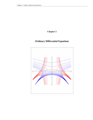
1.3 Initial-value problems and boundary-value problemsAlternatively, we can just draw the velocity curve (a straight line) and calculatethe area under the curve, which is the area of a right triangle:Area 121hours (200 miles/hour) 5/6 miles.12015. a. For any values of A and B, x 3(A Bt)e3t Be3t {3(A Bt) B}e3t (3A B 3Bt)e3t y. Now y 3(3A B 3Bt)e3t 3Be3t (9A 3B 9Bt 3B)e3t (9A 6B 9Bt)e3t and 9x 6y ( 9A 9Bt)e3t (18A 6B 18Bt)e3t (9A 6B 9Bt)e3t , so thaty 9x 6y.b. The initial condition x(0) 1 yields 1 x(0) (A 0)e0 A, and y(0) 0 gives us 0 (3A B), so that B 3. The solution of this system IVPis therefore x(t) (1 3t)e3t , y(t) 9te3t .17. a. Deriving inspiration from Example 1.2.1, we get u(t) u(0)ekat Aekat .b. Substituting the expression for u found in (a) in the differential equakat . If k 0, this last equation istion for w, we get dwdt a(1 k)Aedwjust dt a A, so that w a At C. The condition w(0) 0 tells usthat C 0, so that w(t) aAt. On the other hand, if 0 k 1, thekat and we can integratedifferential equation for w is dwdt a(1 k)Aeekat C. Knowing that w(0) 0, we haveto find that w(t) a(1 k)Akaa(1 k)A (k 1)A. Then we can write0 ka C and therefore C a(1 k)Akak(1 k)(k 1)A(k 1)Akatkatw(t) k Ae k k (1 e ).C kEt kEt CCCe W0 E, then dW 19. a. If W Edt kE W0 E e C kE W E kEW kC k(C EW ).Cb. As t , e kEt 0, so that W (t) E. Note that C/E is in pounds perday. c. From (a) we know that W (t) 250020 180 25002020e 3500 t 125 55e t/175 . A loss of 20 pounds means that W (t) 160, so that we must7 e t/175 .solve the equation 160 125 55e t/175 , 35 55e t/175 , 115

6CHAPTER 1 Introduction to differential equationsTaking the natural logarithm of both sides of this last equation, we getln(7/11) t/175, so that t 175 ln(7/11) 79 days. Similarly, fora loss of 30 pounds, we must solve 150 125 55e t/175 , so that t 175 ln(5/11) 138 days. For a loss of 35 pounds, we solve 145 125 55e t/175 , finding that t 175 ln(4/11) 177 days.Our conclusion is that dieting can be very frustrating. Although it takes 79days to lose the first 20 pounds, it takes an extra 59 days to lose 10 morepounds and 39 additional days to lose 5 pounds beyond the first 30. Theoriginal differential equation indicates that if C and E are constant, withC EW 0, then dW/dt 0 and d 2 W/dt 2 k 2 E(C EW ) 0. Thissays that the weight is a concave up decreasing function of time—that is,the rate of weight loss slows down with time. ktMkAe21. a. y M(1 Ae kt ) 1 y M(1 Ae kt ) 2 · ( kAe kt ) (1 Ae kt )2 kt ktkMAekM1 Ae 1kM11 · · kt kt kt kt kt kt1 Ae1 Ae1 Ae1 Ae1 Ae1 Ae y ky 1 M . Clearly y(0) M/(1 A).387.9802b. Here’s the graph of y(t) 1 54.0812e 0.02270347 t :c.Actual Population1790 3,929,2141980 226,545,8051990 248,709,873Logistic Pop. Value7,043,786225,066,248246,050,716d. limt y(t) limt 23.387.9802 387.9802 million people.1 54.0812e 0.02270347t y ) x(y Suppose y yGR yP . Then x 2 y xy 4y x 2 (yGRP 2 GR 2 yP ) 4(yGR yP ) x yGR xyGR 4yGR x yP xyP 4yP 0 x 3 x 3 . Thus, y, having two arbitrary constants because of its term yGR , is thegeneral solution of the original equation (*).

CHAPTER2First-order differentialequations2.1 Separable equationsA1. dy1 dxA 2yx 2 ln A 2y ln x C1 ln A 2y 2 ln x C2 ln x12 C2 (exponentiating) A 2y Cx 23 , where C3 0 A 2y Cx 24 , where C4 is arbitrary y 12 A Cx 24 AC2 x 2 . Note that C C4 /2 can be any real number if C4 can be any realdydx A 2yx number. 3. y 3 3 y 2 dyA 2ydydt dxx 2 3 y3 dy2y3 3 dt 21y 3 dy 3 1 dt 3y 3 13t C1 y 3 t C2 y (t C2 )3 . Now the initial condition y(2) 0implies that 0 (0 C2 )3 , so that C2 2. Therefore, y (t 2)3 t 3 6t 2 12t 8. But note that in separating the variables we divided by apower of y. The solution y 0 is a singular solution of the basic ODE andsatisfies the initial condition. dydydydx 2 y 2 y cot5. (cot x)y y 2 (cot x) dxx tan x dx 2 y tan x dx ln 2 y ln cos x C1 ln 2 y ln cos x C2 2 y C3 cos x 2 y C4 cos x, so that y 2 C cos x. The initialcondition implies that 1 y(0) 2 C cos(0) 2 C, so that C 3 andy 2 3 cos x. The only possible singular solution is y 2, but this can beobtained by letting C 0. y2 y2dy7. x 2 y 2 y 1 y x 2 y 2 dx y 1 y 1dy dx y 1dy dx x2x2 2 y211y 1 y 1 dy x dx 2 y ln y 1 x C. The constant function y 1 is a singular solution. (We divided by y 1 earlier. Notethat the implicit solution formula is not defined for y 1.) dz xdzdz1x z 9. dx 10x z 10x 10z 10z 10 dx 10z 10 dx ln 10 10ln(C 10x )1x zxxln 10 10 C1 10 10 C z ln 10 ln (C 10 ) z ln 10 .Note that for each particular value of the parameter C, the solution is definedonly for 10x C—that is, for x ln C/ ln 10 (or x log10 C).A Modern Introduction to Differential Equations. Copyright 2021 Elsevier Inc. All rights reserved.7

8CHAPTER 2 First-order differential equations11. (y )2 (x y)y xy 0 (y x)(y y) 0 y x 0 or y y 2dydy x or dx y y x2 C or y Ce x .0 dx13. (x 2y)y 1 y 1dz x 2y . Letting z x 2y, we have dx 1 2y 22z 2z1 x 2y 1 z z . Separating variables, we get z 2 dz dx, or 21 z 2dz dx, and integrating gives us z 2 ln z 2 x C1 . Replacingz by x 2y, we have x 2y 2 ln x 2y 2 x C1 .There is no member of this one-parameter family of solutions that satisfies theinitial condition y(0) 1. However, because we divided by z 2 x 2y 2 in separating variables above, we have a singular solution y (x 2)/2,which also satisfiesthe initialcondition. x 1 y1 y x x 15. y x yx y x 1 yx 1 yx . Now let z y/x. As in the example, y z dz 1 z dz dz x dx , so that the original equation becomes z x dx 1 z , or x dx 1 z1 z21 z1z1 z z 1 z . Separating variables, we get 1 z2 dz 1 z2 1 z2 dz dx12 x . Integrating, we find that arctan z 2 ln 1 z ln x C. Replacing z by 22y/x, we get the solution arctan yx 12 ln x x y ln x C 0.217. y yx . We have a choice here: Let z x/y or z y/x. Because it will dz dymake our work a little easier, we choose z y/x. Now dxallows z x dx 1dydzdzus to write our original equation as dx z x dx 1z z, or x dx z . Sepxy2arating variables and integrating, we find that z2 ln x C1 . Substituting y/x 2for z and multiplying by 2, we get yx 2 ln x C2 , y 2 2x 2 ln x C2 x 2 , so that we have two one-parameter families of solutions: y x 2 ln x Cand y x 2 ln x C. 19. The equation is dB/dt 0.04B, which implies that dB/B 0.04 dt. Thisgives us ln B 0.04t C, B(t) Ke0.04t . Then B(0) 1000 yields the final formula B(t) 1000e0.04t , so B(6) 1000e0.04(6) 1271.25 as the finalbalance.21. The equation is dm/dt 0.0256m. Separating variables, integrating, and exponentiating yield m(t) Ke 0.0256t . We see that m(0) K, the initial masspresent. Thus, m(2) m(0)e 0.0256(2) 0.95K. So we see that after two yearsonly 95% of the original mass is present—i.e., 5% of the original mass has decayed.B x 0ddf (x) dx23. The F TC says that dx0 f (t) dt f (x). Since f (0) 0 f (t) dt 0, we see that we have the IVP y y, y(0) 0. Solving the equation by separating variables, we find that y Cex . The initial condition implies that C 0,so that y f (x) 0.

2.1 Separable equations1 x 2 x 2 dx dt x 1 t C1 x1 t C2 x(t) C t.11Now x(1) 1 1 C 1 C 2 x(t) 2 t .b. The interval I can be as large as ( , 2) or (2, ). Any such interval Icannot include the point t 2, at which x(t) is not defined.c.25. a.dxdt1d. Using the one-parameter formula found in (a), we want 0 x(0) C 0 1C , which is impossible. However, we note that x 0 is a singular solutionthat satisfies the initial condition x(0) 0.dy ln302 (y 20) y 20 ln302 dt ln y 20 ln302 t C1 y ln 2 1/30 t C2 2 t/30 y 20 C3 2 t/30 . Now20 C2 e 30 t C2 eln 2 y(30) 60 60 20 C3 2 30/30 C3 /2, 40 C3 /2 C3 80. There 20 20 80 2 t/30 fore, y 80 2 t/30 20. Now 40 80 2 t/30 ln 141 t/30 ln 1 t ln 2 t 30 24430ln 2 30( 2) 60. 2229. dVdh 16 4 (h 2) dV 16 4 (h 2) dh 164 (h 2)2 dh. Nowlet h 2 2 sin θ , so that dh 2 cos θ dθ . Then we have V 164 4 sin 2 θ · 2 cos θ dθ 16 2 cos θ · 2 cos θ dθ 64 cos2 θ dθ 64 12 θ 14 sin 2θ C 32θ 16 sin 2θ C. Instead of converting back to the variable h, just note that h 0 corresponds to sin θ 1, orθ π/2, and h 4 corresponds to sin θ 1, or θ π/2. Now use the initialcondition to find C: 0 V (0) 32( π/2) 16 sin( π) C, or C 16π.Therefore, V 32θ 16 sin 2θ 16π and V (4) 32(π/2) 16 sin π 16π 32π units. 27.dydt31. a. We have x(t) 0 αβ0 α αβ 1 e(α β)kt(α β)ktβ αe e(α β)kte(α β)ktαβ(α β)kt αβ β αe(α β)kt e αβ(α β)kt αβ β αe(α β)kt e β. (If α β, then α β 0 and 1/e(α β)kt 0 as t .)(α β)kt 0 as t . Therefore, x(t) b. If α α β 0 and e β, thenαβ 1 e(α β)ktβ αe(α β)kt αβ(1 0)β α·0 αββ α as t .9

10CHAPTER 2 First-order differential equations33. We are given db/dt ct, with b(0) 10,000 and b(3) 500,000.a. The solution of the differential equation is b(t) Kect 10,000ect . Theinformation that b(3) 500,000 implies that 500,000 10,000e3c , 50 e3c , ln 50 3c, c (ln 50)/3. Therefore, converting one day into hours,b(24) 10,000e(ln 50/3)·24 10,000 · 508 3.9 1017 cells.b. From part (a), we have b(t) 10,000e(ln 50/3)t , so 20,000 10,000e(ln 50/3)t 2 e(ln 50/3)t ln 2 (ln 50) · t/3 t (3 ln 2)/ ln 50 0.5316 hours 32 minutes.35. We have dm/dt rt and m(1) 0.9m(0). The formula is m(t) m(0)ert ,and m(1) 0.9m(0) implies that 0.9m(0) m(0)er , or 0.9 er . Thus, r ln(0.9), and the formula is complete: m(t) m(0)eln(0.9)t . To calculate thehalf-life, we have m(0)/2 m(0)eln(0.9)t , 1/2 eln(0.9)t , ln(1/2) ln(0.9)t,t ln(1/2)/ ln(0.9) 6.6 years.C37. Let v v(t) denote the velocity of the bullet at time t. Let V be the velocity ofthe bullet at impact, D the final depth of penetrationinto the bale, and T the time required for achieving D. We have dv kv,wherek is a positive constant ofdtproportionality (the “coefficient of friction”). We solve this separable equation2to find that v (C kt), where C is an arbitrary constant. Assuming that v(0) 4V and v(T) 0(boundaryconditions), we can determine the constants k and C: k 2 V /T and C 2 V . Therefore, v V /T 2 (T t)2 . If we let xdenote the distance traveled by the bullet in the bale of cotton, then v dxdt and we can integrate to get x dxV /T 2 (T t)2 dt dt dt v(t) dt V /T 2 (T t)2 dt V /3T 2 (T t)3 C . Because x 0 when t 0,we find that C V T /3. Also note that, because x(T ) D, we have C D( V T /3). In our problem, T 0.1 and D 10. Therefore, V 3D/T 300 ft/sec.39. a. If we let p(x) dy/dx, then dp/dx d 2 y/dx 2 and the original equation 1 2 2.becomes dpdx k 1 p b. Then dp 2 k dx, dp 2 kx C1 , ln p 1 p 2 kx C1 ,1 p 1 pp 1 p 2 C2 ekx . Isolating the radical, squaring both sides, and solvdy C22 ekx 2C1 2 e kx .ing for p, we find that p dx1Integrating with respect to x, we get y C2k2 ekx 2kCe kx C32 1C2 ekx C12 e kx C3 . Note that since the original equation is of 2ksecond order, we get two arbitrary constants in our solution. If we also hadinitial conditions or boundary conditions that would allow us to concludethat C2 1/C2 1 and C3 0, the resulting solution curve would be givenby y 1k cosh(kx), a hyperbolic cosine whose graph is called a catenary.

2.1 Separable equations41. a. The equilibrium solution occurs when μC D 0—that is, whenC Dμ. dC b. Separating variables, we find that μC D dt, which implies that μ1 ln D μC t K1 , ln D μC μt K2 , D μC K3 e μt , K μt . The initial conditionD μC Ke μt , so that C D μμ e KD K0C C0 when t 0 gives us C0 C(0) D μμ e μ , allowingus to conclude that K D μC0 . The final formula for the concentrationD0e μt . As t , e μt 0, so that C(t) Dis C μ D μCμμ 0 Dμ,the equilibrium solution found in part (a).c.43. If r r(t) is the radius of the city at time t and P P (t) is the population, then P απr 2 , travel time T β(2r), and dP /dt γ /T . Thus,d(απr 2 )/dt γ /2βr, so that r 2 dr γ /(4αβπ)dt. So r 3 At B andP C(t E)2/3 . If t 1945 is t0 , then P0 P (t0 ) 5000. If t40 1985,then P4 0 P (t4 0) 20,000. Then 5000 CE 2/3 and 20,000 C(40 E)2/3 .Dividing these last equations, we have 1 40/E 43/2 8, so that E 40/7.If t80 2025, then P (t80 ) C(80 E)2/3 . If we divide by the equation corresponding to t0 , we have P /5000 ((80 E)/E)2/3 (15)2/3 . Therefore,P 5000 · 3 225 30,400 in 2025.11

12CHAPTER 2 First-order differential equations2.2 Linear equationsA 1. y 2y 4x integrating factor μ(x) e 2 dx e2x . Then e2x (y 2y) de2x y 4xe2x e2x y (2x e2x · 4x e2x y 2e2x y e2x 4x dx1)e2x C y 2x 1 Ce 2x . Note that the solution curves are asymptotic to the line y 2x 1 as x tends to infinity. 2 2222det x t 3 et et x t 3 et dt 3. ẋ 2tx t 3 μ(t) e 2t dt et dt t2 222t 1 e2 C x t2 12 Ce t . 5. ty 3y t 3 t 2 ty 3y t 3 t 2 y 3t y t 2 t μ(t) 3 3 653de t dt e3 ln t t 3 dtt y t 5 t 4 t 3 y t6 t5 C y t6 t25 C.t3 7. y x y x cos x xy x 2 cos x xy y x 2 cos x y 1x y 1 yd y x dx e ln x 1/x dxx cos x x x cos x μ(x) ecos x dx sin x C y x sin x Cx. 2 t μ(t) e 1 dt e t e9. t (x x) 1 t 2 et x x 1 tt 1 t 1 t 2 1d t x 2 x t eedtttt t dt ln t t /2 C x et ln t t 2 /2 C . 1x11. xy y ex 0 xy y ex y x1 y ex μ(x) e x dx xd[xy] ex xy ex dx ex C y e x C . The initial conx dxaadition y(a) b implies that b e Ca , so that C ab e and we haveex ab eay(x) . (In the initial condition, clearly a shouldn’t be 0.)x ax ax mx (a m)x axde y e e e13. y ay emx μ(x) e a dx eax dxe y (a m)xe(a m)xedx a m C, if a m 0—that is, if m a. For m a, we emxhave y a m Ce ax . If m a, then eax y e(a a)x dx 1 dx x C,so that y xe ax Ce ax (x C)e ax .[Note: A CAS that can solve ODEs may miss the need for an analysis of twocases.] 1 1 1dtx 1 t 1 t dtt(t 1) e 15. tx t 1 t x t (t 1) x 1 μ(t) e t 1 ln d t 1t 1t 1t 1eln t 1 ln t e t t 1 dtt x t t x t dt t tt· (t ln t C). Now x(1) 0 implies that 0 ln t C x t 1 1t ln1 C),sothatC 1andx(t) (11 1t 1 (t ln t 1).

2.2 Linear equations 17. x ey y 2: Unlike the situation in Exercise 16, just switching the roles ofy and x doesn’t work.equation would not be linear in either x or The resulting e y , we can multiply each side of the differentialy. Noting that e y y equation by e y to get x 1 e y y 2e y . Making the substitution z e y dzdzdzdzgives us x 1 dx 2z, x dx 2z x, and dx 2 2z, x x dxx z 2 1, a linear equation in z. An integrating factor is e x dx x12 . Therefore, dz x12 xz2 x12 dx x1 C z x Cx 2 , or e y we have dxx2 x Cx 2 y ln x Cx 2 .B 19. y 4t y 6ty 2 , or y 4t y 6ty 2 : Here n 2. Divide both sides by y 2 to y 1 6t. Letting z y 1 2 y 1 , we have dzget y 2 y 4 y 2 · dytdt , dt 4dz4so that the equation becomes dzdt t z 6t, or dt t z 6t, linear 4 din z. Now μ(t) e t dt t 4 , so that we have dtt 4 z 6t 5 , t 4 z 6t 5 dt 4t 6 C, y 1z t 6t C . Note that y 0 is a singular solution.t4dy31 3 y 2 and dz 2y 3 dy .dx y xy : Here n 3, so that we let z ydxdx 3 dy y 2 x,Dividing both sides of the original equation by y 3 , we getydx dzdz z x, dx 2z 2x, so that μ(x) e 2 dx e 2x . Thenor 12 dx d 2x z 2xe 2x , or e 2x z 2xe 2x dx 1 e 2x (2x 1) C, sodx e2that z 12 (2x 1) Ce2x x 12 Ce2x and y12 x 12 Ce2x , or 1t 6 C, z 21.y x 12 Ce2x. Note that y 0 is a singular solution. 23. y 2ty ty 2 : Here n 2. Let z y 1 2 y 1 , so that z y 2 y . The original equation becomes z 2tz t. Now μ(t) e 2t dt et et z 2222 222 tet et z tet dt C z e t tet dx Ce t 12 Ce t .Replacing z by y 1 , we get y 1 12 Ce t , y 2212 12 Ce t2 222 1 2Ce t 2et2.2C et25. a.dWdt12221 33 αW 3 βW, dW dt βW αW : Here n 2/3. Letting z W2W 3 and dividing both sides of the ODE by W 3 gives us the new equation21dz1 23 dW3W 3 dW· dt , we can write this lastdt βW α. Noting that dt 3W ββdzdzαequation as 3 dt βz α, or dt 3 z 3 , so that μ(t) e 3 dt βt βtβtβtβtβtde 3 z α3 e 3 e 3 z α3 e 3 dt βα e 3 C z βα e 3 . Now dt13

14CHAPTER 2 First-order differential equationsβt1βt1Ce 3 . Replacing z by W 3 , we find that W 3 βα Ce 3 , or W (t) 3 α βt3.β Ce βt 3b. W limt W (t) limt βα Ce 3 3βt 3 βα C · limt e 3 βα . 3 3c. W (0) 0 0 W (0) βα Ce0 βα C C βα . There 3 βt 3βt 3βt 3fore, W (t) βα βα e 31 e 3 βα W 1 e 3 .d. RR tI E27. a. L dI RI E dI R μ(t) e L dt e L dtdtLL R RRRR tdL tL tL tL tI E e L I Edt E C I dt eLeLeReER Ce RL t. Now the wording of the problem suggests that I (0) 0, so that 0 I (0) ER1 e RLERtb. limt I (t) Ce0 C ER . Therefore, I (t) ER E ReRLt .limt ER1 e RL t ER1 limt e RL t ER.c. By “final” value, we mean the valueE/R found in (b). Nowwe wantI 1E2 R,1R2, Ltor ln1E

In addition to consulting this manual, which contains solutions to all odd-numbered exercises in the text, you should make use of the rich resources of the Internet. You can Google (or use another search engine to locate) any topic in a differential equa- . 1.2 Solutions of differential equations A 1. y sinx,y cosx,y sinx; thus, y y .