Transcription
Solutions Manual (Complete)forDoing Bayesian Data Analysis: A Tutorial with R and BUGSJohn K. KruschkeAcademic Press / Elsevier, 2011. ISBN: 9780123814852Solutions Manual written by John K. KruschkeRevision of March 30, 2011Solutions Manual for Doing Bayesian Data Analysis by John K. KruschkePage 1
Chapter 2.Exercise 2.1. [Purpose: To get you to think about what beliefs can be altered by inferencefrom data.] Suppose I believe that exactly 47 angels can dance on my head. (These angelscannot be seen or felt in any way.) Can you provide any evidence that would change mybelief?No. By assumption, the belief has no observable consequences, and therefore no observable datacan affect the belief.Suppose I believe that exactly 47 anglers can dance on the floor of the bait shop. Is thereany evidence you could provide that would change my belief?Yes. Because dancing anglers and bait–shop floors have measurable spatial extents, data fromobserved anglers and floors can influence the belief.Exercise 2.2. [Purpose: To get you to actively manipulate mathematical models ofprobabilities. Notice, however, that these models have no parameters.] Suppose we have afour–sided die from a board game. (On a tetrahedral die, each face is an equilateraltriangle. When you roll the die, it lands with one face down and the other three visible asthe faces of a three–sided pyramid. To read the value of the roll, you pick up the die andsee what landed face down.) One side has one dot, the second side has two dots, the thirdside has three dots, and the fourth side has four dots. Denote the value of the bottom face asx. Consider the following three mathematical descriptions of the probabilities of x. ModelA: p(x) 1/4. Model B: p(x) x/10. Model C: p(x) 12/(25x). For each model, determine thevalue of p(x) for each value of x. Describe in words what kind of bias (or lack of bias) isexpressed by each model.Model A: p(x 1) 1/4, p(x 2) 1/4, p(x 3) 1/4, p(x 4) 1/4. This model is unbiased, in thatevery value has the same probability.Model B: p(x 1) 1/10, p(x 2) 2/10, p(x 3) 3/10, p(x 4) 4/10. This model is biasedtoward higher values of x.Model C: p(x 1) 12/25, p(x 2) 12/50, p(x 3) 12/75, p(x 4) 12/100. (Notice that theprobabilities sum to 1.) This model is biased toward lower values of x.Exercise 2.3. [Purpose: To get you to think actively about how data cause beliefs to shift.]Suppose we have the tetrahedral die introduced in the previous exercise, along with thethree candidate models of the die‘s probabilities. Suppose that initially we are not surewhat to believe about the die. On the one hand, the die might be fair, with each face landingwith the same probability. On the other hand, the die might be biased, with the faces thathave more dots landing down more often (because the dots are created by embeddingheavy jewels in the die, so that the sides with more dots are more likely to land on thebottom). On yet another hand, the die might be biased such that more dots on a face makeit less likely to land down (because maybe the dots are bouncy rubber or protrude from theSolutions Manual for Doing Bayesian Data Analysis by John K. KruschkePage 2
surface). So, initially, our beliefs about the three models can be described as p(A) p(B) p(C) 1/3. Now we roll the die 100 times and find these results: #1‘s D 25, #2‘s 25, #3‘s 25, and #4‘s 25. Do these data change our beliefs about the models? Which model nowseems most likely?The data are consistent with Model A, which predicts equal numbers of each outcome.Therefore, after observing the data, we should re–allocate belief toward Model A and away fromModel B and Model C. Model A seems most likely.Suppose when we rolled the die 100 times, we found these results: #1‘s 48, #2‘s 24, #3‘s 16, and #4‘s 12. Now which model seems most likely?The data are most consistent with Model C. Therefore, after observing the data, we should re–allocate belief toward Model C and away from Model A and Model B. Model C seems mostlikely.Exercise 2.4. [Purpose: To actually do Bayesian statistics, eventually, and the nextexercises, immediately.] Install R on your computer. (And if that‘s not exercise, I don‘tknow what is.)No written answer needed.Exercise 2.5. [Purpose: To be able to record and communicate the results of your analyses.]Run the code named SimpleGraph.R. The last line of the code saves the graph to a file in aformat called ―encapsulated PostScript‖ (abbreviated as eps), which your favorite wordprocessor might be able to import. If your favorite word processor does not import epsfiles, then read the R documentation and find some other format that your word processorlikes better; try help(‗dev.copy2eps‘). You may find that you can just copy and paste thedisplayed graph directly into your document, but it can be useful to save the graph as astand–alone file for future reference. Include the code listing and the resulting graph in adocument that you compose using a word processor of your choice.The answer depends on individual software preferences. EPS files can be imported into manytypesetting programs, and so no modification to the code is necessary. Some people may findthat storing the file in PDF format is more desirable, in which case the command dev.copy2pdf isuseful instead of dev.copy2eps.Solutions Manual for Doing Bayesian Data Analysis by John K. KruschkePage 3
Exercise 2.6. [Purpose: To gain experience with the details of the command syntax withinR.] Adapt the code of SimpleGraph.R so that it plots a cubic function (y x3) over theinterval x in [–3, 3]. Save the graph in a file format of your choice. Include a listing of yourcode, commented, and the resulting graph.x seq( from –3 , to 3 , by 0.1 )y x 3plot( x , y , type "l" )dev.copy2eps( file "CubicGraph.eps" )####Specify vector of x values.Specify corresponding y values.Make a graph of the x,y points.Save the plot to an EPS file.Solutions Manual for Doing Bayesian Data Analysis by John K. KruschkePage 4
Chapter 3.Exercise 3.1. [Purpose: To give you some experience with random number generation inR.] Modify the coin–flipping program in Section Subsection 3.5.1 (RunningProportion.R)to simulate a biased coin that has p(H) 0.8. Change the height of the reference line in theplot to match p(H). Comment your code. Hint: Read the help for sample.# Goal: Toss a coin N times and compute the running proportion of heads.N 500# Specify the total number of flips, denoted N.# Generate a random sample of N flips for a fair coin (heads 1, tails 0);# the function "sample" is part of R:#set.seed(47405) # Uncomment to set the "seed" for random number generator.flipsequence sample( x c(0,1) , prob c(.2,.8) , size N , replace TRUE )# Compute the running proportion of heads:r cumsum( flipsequence ) # The function "cumsum" is built in to R.n 1:N# n is a vector.runprop r / n# component by component division.# Graph the running proportion:# To learn about the parameters of the plot function,# type help('par') at the R command prompt.# Note that "c" is a function in R.plot( n , runprop , type "o" , log "x" ,xlim c(1,N) , ylim c(0.0,1.0) , cex.axis 1.5 ,xlab "Flip Number" , ylab "Proportion Heads" , cex.lab 1.5 ,main "Running Proportion of Heads" , cex.main 1.5 )# Plot a dotted horizontal line at y .8, just as a reference line:lines( c(1,N) , c(.8,.8) , lty 2 , lwd 2 )# Display the beginning of the flip sequence. These string and character# manipulations may seem mysterious, but you can de–mystify by unpacking# the commands starting with the innermost parentheses or brackets and# moving to the outermost.flipletters paste( c("T","H")[ flipsequence[ 1:10 ] 1 ] , collapse "" )displaystring paste( "Flip Sequence " , flipletters , "." , sep "" )text( 5 , .9 , displaystring , adj c(0,1) , cex 1.3 )# Display the relative frequency at the end of the sequence.text( N , .3 , paste("End Proportion ",runprop[N]) , adj c(1,0) , cex 1.3 )# Save the plot to an EPS file.dev.copy2eps( file "Exercise3.1.eps" )Below is an exemplary graph; displays will differ across runs because the flip sequence israndom.Solutions Manual for Doing Bayesian Data Analysis by John K. KruschkePage 5
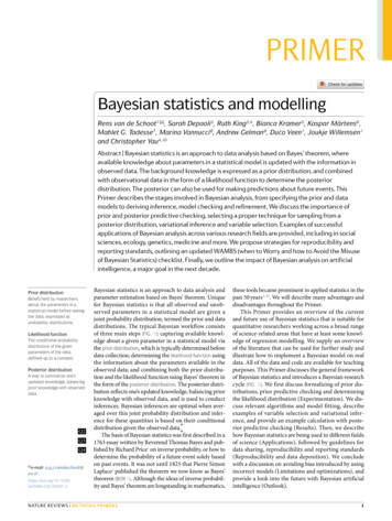
Exercise 3.2. [Purpose: To have you work through an example of the logic presented inSection 3.2.1.2.] Determine the exact probability of drawing a 10 from a shuffled pinochledeck. (A pinochle deck has 48 cards. There are six values: 9, 10, jack, queen, king, and ace.There are two copies of each value in each of the standard four suits: hearts, diamonds,clubs, and spades.)(A) What is the probability of getting a 10?There are 8 10’s in 48 cards, hence p(10) 8/48.(B) What is the probability of getting a 10 or jack?There are 8 10’s and 8 jacks and they are mutually exclusive. Hence p(10 or jack) (8 8)/48.Exercise 3.3. [Purpose: To give you hands–on experience with a simple probability densityfunction, in R and in calculus, and to reemphasize that density functions can have valueslarger than 1.] Consider a spinner with a [0,1] scale on its circumference. Suppose that thespinner is slanted or magnetized or bent in some way such that it is biased, and itsprobability density function is p(x) 6x(1–x) over the interval x in [0, 1].(A) Adapt the code from Section Subsection 3.5.2 (IntegralOfDensity.R) to plot this densityfunction and approximate its integral. Comment your code. Be careful to consider values ofx only in the interval [0, 1]. Hint: You can omit the first couple lines regarding meanvaland sdval, because those parameter values pertain only to the normal distribution. Then setxlow 0 and xhigh 1.Solutions Manual for Doing Bayesian Data Analysis by John K. KruschkePage 6
# Graph of normal probability density function, with comb of intervals.xlow 0 # Specify low end of x–axis.xhigh 1 # Specify high end of x–axis.dx 0.02# Specify interval width on x–axis# Specify comb points along the x axis:x seq( from xlow , to xhigh , by dx )# Compute y values, i.e., probability density at each value of x:y 6 * x * ( 1 – x )# Plot the function. "plot" draws the intervals. "lines" draws the curve.plot( x , y , type "h" , lwd 1 , cex.axis 1.5, xlab "x" , ylab "p(x)" , cex.lab 1.5, main "6x(1–x)" , cex.main 1.5 )lines( x , y )# Approximate the integral as the sum of width * height for each interval.area sum( dx * y )# Display info in the graph.text( 0.8 , .9*max(y) , bquote( paste(Delta , "x " ,.(dx)) ), adj c(0,.5) )text( 0.8 , .8*max(y) ,bquote(paste( sum(,x,) , " " , Delta , "x p(x) " , .(signif(area,3)) )) , adj c(0,.5) )# Save the plot to an EPS file.dev.copy2eps( file "Exercise3.3.eps" )(B) Derive the exact integral using calculus. Hint: See the example, Equation 3.7.12 1 3 6 1 2 1 3 1 2 1 3 121dx(6x(1 x)) 6dx(x x) 6[ 2 x 3 x ]0 [ 2 1 31 ] [ 2 0 3 0 ] 0 011Solutions Manual for Doing Bayesian Data Analysis by John K. KruschkePage 7
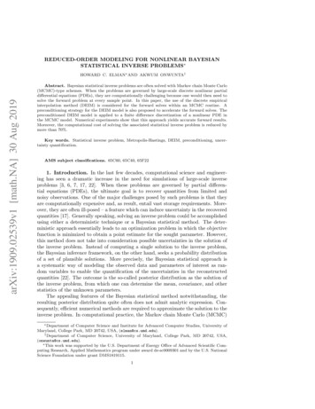
(C) Does this function satisfy Equation 3.3?Yes, the integral of the function across its domain is 1, just as it should be for a probabilitydensity function.(D) From inspecting the graph, what is the maximal value of p(x)?Visual inspection of the graph suggests that p(x) is maximal at x 0.5. This is also the mean,because the distribution is symmetric.Exercise 3.4. [Purpose: To have you use a normal curve to describe beliefs. It‘s also handyto know the area under the normal curve between and .](A) Adapt the code from Section Subsection 3.5.2 (IntegralOfDensity.R) to determine(approximately) the probability mass under the normal curve from x – to x .Comment your code. Hint: Just change xlow and xhigh appropriately, and change the textlocation so that the area still appears within the plot.# Graph of normal probability density function, with comb of intervals.meanval 0.0# Specify mean of distribution.sdval 0.2# Specify standard deviation of distribution.xlow meanval – 1*sdval # Specify low end of x–axis.xhigh meanval 1*sdval # Specify high end of x–axis.dx 0.002# Specify interval width on x–axis# Specify comb points along the x axis:x seq( from xlow , to xhigh , by dx )# Compute y values, i.e., probability density at each value of x:y ( 1/(sdval*sqrt(2*pi)) ) * exp( –.5 * ((x–meanval)/sdval) 2 )# Plot the function. "plot" draws the intervals. "lines" draws the bellcurve.plot( x , y , type "h" , lwd 1 , cex.axis 1.5, xlab "x" , ylab "p(x)" , cex.lab 1.5, main "Normal Probability Density" , cex.main 1.5 )lines( x , y )# Approximate the integral as the sum of width * height for each interval.area sum( dx * y )# Display info in the graph.text( –0.5*sdval , .95*max(y) , bquote( paste(mu ," " ,.(meanval)) ), adj c(1,.5) )text( –0.5*sdval , .9*max(y) , bquote( paste(sigma ," " ,.(sdval)) ), adj c(1,.5) )text( 0.5*sdval , .95*max(y) , bquote( paste(Delta , "x " ,.(dx)) ), adj c(0,.5) )text( 0.5*sdval , .9*max(y) ,bquote(paste( sum(,x,) , " " , Delta , "x p(x) " , .(signif(area,3)) )) , adj c(0,.5) )# Save the plot to an EPS file.dev.copy2eps( file "Exercise3.4.eps" )Solutions Manual for Doing Bayesian Data Analysis by John K. KruschkePage 8
The graph indicates that the area under the normal curve between and is about 34%.(B) Now use the normal curve to describe the following belief. Suppose you believe thatwomen‘s heights follow a bell–shaped distribution, centered at 162 cm with about two–thirds of all women having heights between 147 cm and 177 cm.The previous part indicates that about two–thirds of the normal distribution falls between – and Therefore we can describe the belief as a normal distribution with mean at 162 andstandard deviation of 177–162 15 (which is the same as 162–147).Exercise 3.5. [Purpose: To recognize and work with the fact that Equation 3.11 can besolved for the conjoint probability, which will be crucial for developing Bayes‘ theorem.]School children were surveyed regarding their favorite foods. Of the total sample, 20%were 1st graders, 20% were 6th graders, and 60% were 11th graders. For each grade, thefollowing table shows the proportion of respondents that chose each of three foods as theirfavorite:Ice Cream1st graders 0.36th graders 0.611th graders 0.3Fruit0.60.30.1French Fries0.10.10.6From that information, construct a table of conjoint probabilities of grade and favoritefood. Also, say whether grade and favorite food are independent and how you ascertainedthe answer. Hint: You are given p(grade) and p(food grade). You need to determinep(grade, food).Solutions Manual for Doing Bayesian Data Analysis by John K. KruschkePage 9
By definition, p(food grade) p(grade,food)/p(grade). Therefore p(grade,food) p(food grade)*p(grade). Therefore we multiply each row of the table by its correspondingmarginal distribution to get the conjoint probabilities:1st graders6th graders11th gradersIce Cream0.3*0.2 0.060.6*0.2 0.120.3*0.6 0.18Fruit0.6*0.2 0.120.3*0.2 0.060.1*0.6 0.06French Fries0.1*0.2 0.020.1*0.2 0.020.6*0.6 0.36If the attributes were independent, then we could multiply the marginal probabilities to get theconjoint probabilities. Any cell that violates that equality indicates lack of independence.Consider, for example, the top left cell. Its conjoint probability is p(1stGrade,IceCream) 0.06.On the other hand, the product of the marginals is p(1stGrade) * p(IceCream) 0.20 * 0.36 0.072, which does not equal the conjoint probability.Solutions Manual for Doing Bayesian Data Analysis by John K. KruschkePage 10
Chapter 4.Exercise 4.1. [Purpose: Application of Bayes‘ rule to disease diagnosis, to see the importantrole of prior probabilities.] Suppose that in the general population, the probability ofhaving a particular rare disease is 1 in a 1000. We denote the true presence or absence ofthe disease as the value of a parameter, , that can have the value if disease ispresent, or the value if the disease is absent. The base rate of the disease is thereforedenoted p( ) 0.001. This is our prior belief that a person selected at random has thedisease.Suppose that there is a test for the disease that has a 99% hit rate, which means that if aperson has the disease, then the test result is positive 99% of the time. We denote a positivetest result as D and a negative test result as D –. The observed test result is a bit ofdata that we will use to modify our belief about the value of the underlying diseaseparameter. The hit rate is expressed as p( D ) 0.99. The test also has a falsealarm rate of 5%. This means that 5% of the time when the disease is not present, the testfalsely indicates that the disease is present. We denote the false alarm rate as p( D ) 0.05.Suppose we sample a person at random from the population, administer the test, and itcomes up positive. What is the posterior probability that the person has the disease?Mathematically expressed, we are asking, what is p( D )? Before determining theanswer from Bayes‘ rule, generate an intuitive answer and see if your intuition matches theBayesian answer. Most people have an intuition that the probability of having the disease isnear the hit rate of the test (which in this case is 0.99).Hint: The following table of conjoint probabilities might help you understand the possiblecombinations of events. (The following table is a specific case of Table 4.2, p. 57.) The priorprobabilities of the disease are on the bottom marginal. When we know that the test resultis positive, we restrict our attention the row marked D .[The table is not reproduced here.]By Bayes’ rule,p( D ) p(D ) p( ) / p(D ) p(D ) p( ) / [ p(D ) p( ) p(D ) p( ) ] 0.99 * 0.001 / [ 0.99 * 0.001 0.05 * 0.999 ] 0.0194 (rounded to three significant digits)Thus, despite the high hit rate of the test, the small prior and non–negligible false–alarm ratemake the posterior probability less than 2%. (This analysis assumes that there were no othersymptoms and that the person was selected at random so that the prior is applicable.)Solutions Manual for Doing Bayesian Data Analysis by John K. KruschkePage 11
Exercise 4.2. [Purpose: Iterative application of Bayes‘ rule, to see how posteriorprobabilities change with inclusion of more data.] Continuing from the previous exercise,suppose that the same randomly selected person as in the previous exercise is retested afterthe first test comes back positive, and on the retest the result is negative. Now what is theprobability that the person has the disease? Hint: For the prior probability of the retest,use the posterior computed from the previous exercise. Also notice thatp(D – ) 1 – p(D ) and p(D – ) 1 – p(D ).To avoid rounding error, it is important to retain many significant digits for the prior. From theprevious exercise, p( ) 0.0194346289753. Then, by Bayes’ rule,p( D – ) p(D – ) p( ) / p(D –) p(D – ) p( ) / [ p(D – ) p( ) p(D – ) p( ) ]where p( ) is the posterior from the previous exercise. Hencep( D – ) (1–0.99)*0.0194 / [ (1–0.99)*0.0194 (1–.05)*( 1–0.0194 ) ] 0.000209 (rounded to three significant digits)Exercise 4.3. [Purpose: To get an intuition for the previous results by using ―naturalfrequency‖ and ―Markov‖ representations.](A) Suppose that the population consists of 100,000 people. Compute how many peopleshould fall into each cell of the table in the hint shown in Exercise 4.1. To compute theexpected frequency of people in a cell, just multiply the cell probability by the size of thepopulation. To get you started, a few of the cells of the frequency table are filled in [below]. Your job for this part of the exercise is to fill in the frequencies of the remaining cells ofthe table.D D –θ freq(D , ) p(D , ) N p(D ) p( ) N .99 * .001 * 100000 99freq(D – , ) p(D – , ) N p(D – ) p( ) N (1-.99) * .001 * 100000 1100θ freq(D , ) p(D , ) N p(D ) p( ) N .05 * (1-.001) * 100000 4,995freq(D – , ) p(D – , ) N p(D – ) p( ) N (1-.05) * (1-.001) * 100000 94,90599,9005,09494,906N 100,000(B) Take a good look at the frequencies in the table you just computed for the previouspart. These are the so-called ―natural frequencies‖ of the events, as opposed to thesomewhat unintuitive expression in terms of conditional probabilities (Gigerenzer &Hoffrage, 1995). From the cell frequencies alone, determine the proportion of people whohave the disease, given that their test result is positive. Before computing the exact answerSolutions Manual for Doing Bayesian Data Analysis by John K. KruschkePage 12
arithmetically, first give a rough intuitive answer merely by looking at the relativefrequencies in the row D . Does your intuitive answer match the intuitive answer youprovided back in Exercise 4.1? Probably not. Your intuitive answer here is probably muchcloser to the correct answer. Now compute the exact answer arithmetically. It should matchthe result from applying Bayes‘ rule in Exercise 4.1.The result is positive, so we focus attention on the row D , which has a total of 5,094 peopleof whom 99 have the disease. Hencep( D ) 99 / 5094 0.01943463This exactly matches the result of Exercise 4.1.(C) Now we‘ll consider a related representation of the probabilities in terms of naturalfrequencies, which is especially useful when we accumulate more data. Krauss, Martignon,& Hoffrage (1999) called this type of representation a ―Markov‖ representation. Supposenow we start with a population of N D 10,000,000 people. We expect 99.9% of them (i.e.,9,990,000) not to have the disease, and just 0.1% (i.e., 10,000) to have the disease. Nowconsider how many people we expect to test positive. Of the 10,000 people who have thedisease, 99% (i.e., 9900), will be expected to test positive. Of the 9,990,000 people who donot have the disease, 5%, (i.e., 499,500) will be expected to test positive. Now considerretesting everyone who has tested positive on the first test. How many of them are expectedto show a negative result on the retest? Use this diagram to compute your answer:(D) Use the diagram in the previous part to answer this question: What proportion ofpeople who test positive at first and then negative on retest actually have the disease? Inother words, of the total number of people at the bottom of the diagram in the previouspart (those are the people who tested positive then negative), what proportion of them arein the left branch of the tree? How does the result compare with your answer to Exercise4.2?Notice that the total of the bottom is 99 474,525 474,624 people who test positive andnegative. The proportion of those who actually have the disease is 99 / 474,624 0.000209(rounded to three significant digits). This matches the result from Exercise 4.2.Solutions Manual for Doing Bayesian Data Analysis by John K. KruschkePage 13
Exercise 4.4. [Purpose: To see a hands-on example of data-order invariance.] Consideragain the disease and diagnostic test of the previous two exercises. Suppose that a personselected at random from the population gets the test and it comes back negative. Computethe probability that the person has the disease. The person then is retested, and on thesecond test the result is positive. Compute the probability that the person has the disease.How does the result compare with your answer to Exercise 4.2?As noted in the answer to Exercise 4.2, retention of many significant digits is important to avoidrounding error.After the first (negative) test,p( D – ) p(D – ) p( ) / p(D –) p(D – ) p( ) / [ p(D – ) p( ) p(D – ) p( ) ] (1–0.99)*0.001 / [ (1–0.99)*0.001 (1–.05)*( 1–0.001 ) ] 0.0000105367416180After the second (positive) test,p( D ) p(D ) p( ) / p(D ) p(D ) p( ) / [ p(D ) p( ) p(D ) p( ) ] 0.99 * 0.0000105 / [ 0.99 * 0.0000105 0.05 * (1-0.0000105 ) ] 0.000209 (rounded to three significant digits)This result matches the previous exercises.Exercise 4.5. [Purpose: An application of Bayes‘ rule to neuroscience, to infer cognitivefunction from brain activation.] Cognitive neuroscientists investigate which areas of thebrain are active during particular mental tasks. In many situations, researchers observethat a certain region of the brain is active and infer that a particular cognitive function istherefore being carried out. Poldrack (2006) cautioned that such inferences are notnecessarily firm and need to be made with Bayes‘ rule in mind. Poldrack (2006) reportedthe following frequency table of previous studies that involved any language-related task(specifically phonological and semantic processing) and whether or not a particular regionof interest (ROI) in the brain was activated:Language StudyActivated166Not activated 703Not Language Study1992154Suppose that a new study is conducted and finds that the ROI is activated. If the priorprobability that the task involves language processing is 0.5, what is the posteriorprobability, given that the ROI is activated? (Hint: Poldrack (2006) reports that it is 0.69.You job is to derive this number.)p( Lang. ROI Act. ) p( ROI Act. Lang. ) p( Lang. )/ (p(ROI Act. Lang.) p(Lang.) p(ROI Act. NotLang.) p(NotLang.) ) 166/(166 703)*0.5 / (166/(166 703)*0.5 199/(199 2154)*0.5 ) 0.693Notice that the posterior probability of involving language is only a little higher than the prior.Solutions Manual for Doing Bayesian Data Analysis by John K. KruschkePage 14
Exercise 4.6. [Purpose: To make sure you really understand what is being shown in Figure4.1.] Derive the posterior distribution in Figure 4.1 by hand. The prior has p( .25) .25,p( .50) .50, and p( .75) .25. The data consist of a specific sequence of flips withthree heads and nine tails, so p(D ) 3(1- . Hint: Check that your posteriorprobabilities sum to 1.p( .25 D) p(D .25) p( .25)/ [p(D .25) p( .25) p(D .50) p( .50) p(D .75) p( .75) ] .253(1-.25)9*.25/ [ .253(1-.25)9*.25 .503(1-.50)9*.50 .753(1-.75)9*.25 ] 0.705Similarly, p( .50 D) 0.294 and p( .75 D) 0.001.(For future reference, the denominator in the equation above is 0.0004158, rounded to foursignificant digits.)Exercise 4.7. [Purpose: For you to see, hands on, that p(D) lives in the denominator ofBayes‘ rule.] Compute p(D) in Figure 4.1 by hand. Hint: Did you notice that you alreadycomputed p(D) in the previous exercise?p(D) p(D .25) p( .25) p(D .50) p( .50) p(D .75) p( .75)which is the denominator from the previous exercise, where we found that p(D) 0.0004158.Solutions Manual for Doing Bayesian Data Analysis by John K. KruschkePage 15
Chapter 5.Exercise 5.1. [Purpose: To see the influence of the prior in each successive flip, and to seeanother demonstration that the posterior is invariant under reorderings of the data.] Forthis exercise, use the R function of Section 5.5.1 (BernBeta.R). (Read the comments at thetop of the code for an example of how to use it, and don‘t forget to source the functionbefore calling it.) Notice that the function returns the posterior beta values each time it iscalled, so you can use the returned values as the prior values for the next function call.(A) Start with a prior distribution that expresses some uncertainty that a coin is fair:beta( 4, 4). Flip the coin once; suppose we get a head. What is the posterior distribution?At the R command prompt, typingpost BernBeta( c(4,4) , c(1) )yields this figure:(The jagged bits in the curve are artifacts of how Microsoft Word incorrectly renders EPSfigures. The curves are actually smooth.)Solutions Manual for Doing Bayesian Data Analysis by John K. KruschkePage 16
(B) Use the posterior from the previous flip as the prior for the next flip. Suppose we flipagain and get a head. Now what is the new posterior? (Hint: If you type post BernBeta(c(4,4) , c(1) ) for the first part, then you can type post BernBeta( post , c(1) ) for the nextpart.)At the R command prompt, typingpost BernBeta( post , c(1) )yields this figure:(The jagged bits in the curve are artifacts of how Microsoft Word incorrectly renders EPSfigures. The curves are actually smooth.)Solutions Manual for Doing Bayesian Data Analysis by John K. KruschkePage 17
(C) Using that posterior as the prior for the next flip, flip a third time and get T. Now whatis the new posterior? (Hint: Type post BernBeta( post , c(0) ).)At the R command prompt, typingpost BernBeta( post , c(0) )yields this figure:(The jagged bits in the curve are artifacts of how Microsoft Word incorrectly renders EPSfigures. The curves are actually smooth.)Solutions Manual for Doing Bayesian Data Analysis by John K. KruschkePage 18
(D) Do the same three updates but in the order T, H, H instead of H, H, T. Is the finalposterior distribution the same for both orderings of the flip results?The sequence of commands ispost BernBeta( c(4,4) , c(0) )post BernBeta( post , c(1) )post BernBeta( post , c(1) )and the final graph looks like this:Notice that the ultimate posterior is the same as Part C, but the prior leading up to it is differentbecause of the different sequence of updating. (The jagged bits in the curve are artifacts of howMicrosoft Word incorrectly renders EPS figures. The curves are actually smooth.)Solutions Manual for Doing Bayesian Data Analysis by John K. KruschkePage 19
Exercise 5.2. [Purpose: To connect HDIs to the real world, with iterative data collection.]Suppose an election is approaching, and you are interested in knowing whether the generalpopulation prefers candidate A or candidate B. A just published poll in the newspapers
Solutions Manual for Doing Bayesian Data Analysis by John K. Kruschke Page 4 Exercise 2.6. [Purpose: To gain experience with the details of the command syntax within R.] Adapt the code of SimpleGraph.R so that it plots a cubic function (y x3) over the interval x in [-3, 3].Save the graph in a file format of your choice.