Transcription
Distributed OptimalControl of MultiscaleDynamical SystemsA TutorialSilvia Ferrari, Greg Foderaro,Pingping Zhu,and Thomas A. WettergrenMany complex systems, ranging from renewable resources [1] to very-large-scalerobotic systems (VLRS) [2], can be described as multiscale dynamical systemscomprising many interactive agents. In recent years, significant progress hasbeen made in the formation control and stability analysis of teams of agents,such as robots, or autonomous vehicles. In these systems, the mutual goals ofthe agents are, for example, to maintain a desired configuration, such as a triangle or a starformation, or to perform a desired behavior, such as translating as a group (schooling) ormaintaining the center of mass of the group (flocking) [2]–[7]. While this literature has successfully illustrated that the behavior of large networks of interacting agents can be conveniently described and controlled by density functions, it has yet to provide an approach foroptimizing the agent density functions such that their mutual goals are optimized.Digital Object Identifier 10.1109/MCS.2015.2512034Date of publication: 17 March 2016102 IEEE CONTROL SYSTEMS MAGAZINE»april 20161066-033X/16 2016ieee
TABLE 1 Distributed optimal control notation.SymbolMeaningiAgent indexxAgent microscopic stateuAgent controlUAdmissible control spacepAgent distributionp)Optimal agent distributiontpEstimated agent distributionJIntegral cost functionLLagrangian functionzTerminal cost functionT0Initial timeTfFinal timedGradient (column) vectorfijth Gaussian mixture component jWeight of the jth Gaussian mixture componentnjMean of the jth Gaussian mixture component/jCovariance matrix of the jth Gaussian mixturecomponentzNumber of Gaussian mixture componentstkFV approximation of advection operator3 t, 3 xTemporal and spatialdiscretization intervalsK, LNumber of temporal and spatial collocation pointsmLagrange multiplier or costate vectorKKernel functionH i, k, c i, kBandwidth matrix and weighting coefficient ofkernel k stored by agent iUPotential functionU repRepulsive potential functionThis article describes a coarse-grained optimal controlapproach for multiscale dynamical systems, referred to asdistributed optimal control (DOC), which enables the optimization of density functions, and/or their moments, subject to the agents’ dynamic constraints. (See Table 1 for DOCnotation.) The DOC approach is applicable to systems, suchas swarms or teams, composed of many collaborative agentsthat, on small spatial and time scales, are each described bya small set of ordinary differential equations (ODEs)referred to as the microscopic or detailed equations. Onlarger spatial and temporal scales, the agent behaviors andinteractions are assumed to give rise to macroscopic coherent behaviors, or coarse dynamics, described by partial differential equations (PDEs) that are possibly stochastic.In recent years, the optimal control of stochastic differential equations (SDEs) has gained increasing attention.Considerable research efforts have focused on the optimalcontrol and estimation of SDEs driven by non-Gaussianprocesses, such as Brownian motion combined with Poisson processes, or other stochastic processes [8]–[10]. Inthese efforts, the microscopic agent state is viewed as arandom vector, and the dynamic equation takes the form ofan SDE that describes the evolution of the statistics of themicroscopic vector function and may be integrated usingstochastic integrals. Then, the performance of N agents isexpressed as an integral function of N vector fields to beoptimized subject to N SDEs. However, solutions can onlybe obtained for relatively few and highly idealized cases inwhich finite-dimensional, local approximations can beconstructed, for example, via moment closure [8], [9]. Whilethe optimal control of SDEs has been primarily shownuseful to selected applications in population biology andfinance [8]–[10], recently it has also been successfullyapplied to obtain equilibrium strategies for multiagent systems (MAS) that obey a game-theoretic framework whereeach agent has its own cost function and the macroscopicsystem performance is expressed by a predefined collectivepotential function (see [11] and the references therein).Other approaches that have been proposed for tacklingthe control of multiscale dynamical systems and providepractical yet tractable solutions even when the number ofagents is large include prioritized planning techniques [12]and path-coordination methods [13], which first planthe agent trajectories independently and then adjustthe microscopic control laws to avoid mutualcollisions. Behavior-based control methodsseek feasible solutions by programming a set of simple behaviors for eachagent and by showing that the agents’interactions give rise to a macroscopicbehavior, such as dispersion [2]. Swarmintelligence methods, such as foragingand schooling [5], [14], [15], view eachagent as an interchangeable unit subject to local objectives and constraintsthrough which the swarm can converge to a range of predefined distributions or a satisfactory strategy. Whenthe agents’ dynamics and costs areweakly coupled, useful decentralizedcontrol strategies for multiscale dynamical systems can be obtained viathe Nash certainty equivalence (NCE) ormean field principle [16], [17].Similarly to DOC, NCE methods rely onidentifying a consistency relationship betweenthe microscopic agent dynamics and a macroscopicdescription, which in the NCE is the mass of the agents.However, while in NCE methods the (weak) couplingsapril 2016« IEEE CONTROL SYSTEMS MAGAZINE103
between agents are produced by averaging the microscopicagent dynamics and costs, in DOC couplings need not beweak, and may arise as a result of collaborative objectivesexpressed by the macroscopic cost function. As a result, thecost function can represent objectives of a far more generalform than other methods and admit solutions that entailstrong couplings between the agent dynamics and controllaws. Furthermore, while NCE methods rely on a macroscopic state description defined in terms of the expectation(or mean) of the evolving agent distribution, the DOCapproach is applicable to other macroscopic descriptions,such as the agent probability density function (PDF) and itsmoments, thereby admitting a wide range of collaborativebehaviors and objectives.Unlike prioritized and path-coordination methods [12],[13], the DOC approach does not rely on decoupling theagent behaviors, or on specifying the agent distribution apriori. Instead, DOC optimizes the macroscopic behaviorof the system subject to coupled microscopic agent dynamics and relies on the existence of an accurate macroscopicevolution equation and an associated restriction operatorthat characterize the multiscale system to reduce the computational complexity of the optimal control problem. As aresult, the computation required is far reduced comparedto classical optimal control [18], and coupled agent objectives and control laws can be considered over large spatialand time scales without sacrificing optimality or completeness [19].This tutorial provides an introductory overview of theDOC problem and of how it compares to existing optimalcontrol methods. Two existing DOC solution methods aredescribed, and the necessary and sufficient conditions foroptimality are reviewed in the context of direct and indirect DOC methods. Similarly to classical optimal control,indirect DOC methods seek to determine solutions to theoptimality conditions [20]. Direct DOC methods discretizethe original problem formulation, in this case both withrespect to space and time, to obtain a mathematical program that, in the general case, takes the form of a nonlinearprogram (NLP). Subsequently, each agent can compute itsfeedback control law based on the optimal time-varyingagent PDF determined by DOC and on the actual agent distribution, which may be obtained via kernel density estimation. Finally, the applicability of the DOC approach isillustrated through a multiagent formation and path-planning application and an image-reconstruction problem.Background on Optimal ControlOptimal control can be considered the most general approachto optimizing the performance of a dynamical system overtime. Over the years, it has been successfully applied to control a wide range of processes, including physical, chemical,economic, and transportation systems. The classical optimalcontrol formulation considers a system whose dynamics canbe approximated by a small system of SDEs104 IEEE CONTROL SYSTEMS MAGAZINE»april 2016xo (t) f [x (t), u (t), t] G (t) w (t), x (T0) x 0, (1)where x and u are the system state and control input vectors,respectively, and w ! R s is a vector of random inputs withGaussian distribution and zero mean [21]. The dynamics in(1) also depend on system parameters that represent thephysical characteristics of the system and are expressed inunits that scale both the inputs and outputs to comparablemagnitudes. The term G (t) w (t) is typically assumed to capture the random effects associated with parameter variationsand uncontrollable inputs known as disturbances [21, p. 422].Classical optimal control seeks to determine the state andcontrol trajectories that optimize an integral cost functionTfJ z [x (T f )] #L [x (t), u (t), t] dt, (2)T0over a time interval (T0, T f ], subject to (1) and, potentially,to an d-dimensional inequality constraintq [x (t), u (t), t] # 0 d # 1 . (3)When random effects can be neglected, optimal controlproblems in the form (1)–(3) can be approached by solvingthe necessary conditions for optimality known as Euler–Lagrange equations, which may be derived using calculusof variations [21]. Another approach is to use the recurrencerelationship of dynamic programming to iterativelyapproximate candidate optimal trajectories, known asextremals, by optimizing the value function or cost-to-go.For a nonlinear system and a general cost function, theEuler–Lagrange equations amount to a Hamiltonianboundary-value problem for which there typically are noclosed-form solutions. In this case, the optimal controlproblem is typically solved numerically using direct orindirect methods [21]–[23].Indirect methods solve a nonlinear multipoint boundary value problem to determine candidate optimal trajectories. This requires deriving analytical expressions for thenecessary conditions for optimality and then implementing a root-finding algorithm to solve the optimality conditions numerically. Direct methods determine near-optimalsolutions by discretizing the continuous-time problemabout collocation points and then transcribing it into afinite-dimensional NLP. A numerical optimization algorithm, such as sequential quadratic programming (SQP), isthen used to find the optimal dynamic state and controlvariables directly from the discretized optimal controlproblem [24], [25]. Direct methods are typically easier toimplement than indirect methods because they do notinvolve the derivation of analytical expressions, which maybe challenging especially for nonlinear systems, havebetter convergence properties, and do not require initialguesses for the adjoint variables, which can be difficult toprovide in the presence of inequality constraints [26]–[28].When random effects are too important to be neglected,the stochastic principle of optimality can be obtained by
taking the expectation of the integral cost (2), ultimatelyreducing the stochastic optimal control problem to the minimization of a value function that differs from its deterministic counterpart by a term containing the spectral densitymatrix of the random input [21, pp. 422–432]. Traditionally,stochastic optimal control has dealt with a single dynamicalsystem modeled by a small system of ODEs with additiveGaussian random inputs, such as (1). In recent years, however, considerable efforts have gone into the optimal controland estimation of stochastic differential equations drivenby non-Gaussian processes such as Brownian motion andPoisson processes [8]–[11]. Let the state of the ith agent berepresented by a random vector, x i, subject to a stochasticprocess that takes the form of the SDEdx i (t) {f [x i (t), t] Bu i (t)} dt G [x i (t), t] dw i (t), x i (t 0) x i0,(4)where w i denotes a Brownian motion process [11]. Then,the performance of N agents can be expressed as an integral function of f [x 1 (t)], f, f [x N (t)], and must be optimizedsubject to N SDEs in the form of (4), which can be integrated using stochastic integrals. While this approachallows modeling and optimizing stochastic processes thatare not well described by ODEs with additive Gaussian distributions, it does not resolve the computational challengesassociated with many collaborative agents. In fact, the optimal control of SDEs, such as (4), typically requires solvingoptimality conditions that are numerically more challenging than the Euler–Lagrange equations and do not affordany computational savings.In many MAS, the goal is to control processes that caneach be described by the ODEs in (1) but, because of commongoals and objectives, ultimately lead to coupled optimalityconditions and emergent behaviors governed by PDEs. Todate, the control of PDEs or distributed-parameter systemshas focused primarily on parabolic models, such as2X N {X (z, t)} U (z, t), z ! D, t 0,2t B {X (z, t)} 0, z ! 2D, X (z, 0) X 0 (z), z ! D,(5)where z [x y] T are the coordinates of the spatial domainD ! R 2 with boundary denoted by 2D, N { } and B { } arewell-posed linear or nonlinear spatial differential operators,X 0 is a known function, and U (z, t) is the forcing function orcontrol input to be determined. In a typical distributedparameter system, the scalar input U can be used to controlthe spatial and temporal evolution of the state X and can bedesigned to be a function of X via feedback [29]. Thus, optimal control of PDEs seeks to optimize an integral cost function of X and U over a domain D, subject to a PDE such as(5). The solution to this class of distributed control problemscan be obtained from the Karush–Kuhn–Tucker (KKT) conditions, as described in detail in [29].The methods reviewed above show that optimal controlis a promising framework for controlling the behavior ofMAS because it enables the optimization of integral costfunctions in dynamic and uncertain settings. Like many ofthe aforementioned methods, DOC seeks to extend optimal control theory to new problem formulations that arenot restricted to systems described by ODEs. In particular,DOC addresses the optimization of restriction operatorsthat capture the macroscopic performance of a multiscaledynamical system by means of a reduced-order representation of the agents’ state that is governed by PDEs. TheDOC methods reviewed in this article focus on the optimal control of time-varying PDFs subject to a parabolicPDE known as the advection-diffusion equation, whichcan be obtained from (5) by considering multivariable stateand control and vector-valued operators N { } and B { } .Unlike existing methods for the control of parabolic PDEs,DOC considers multiscale systems in which agents havemicroscopic control inputs and dynamics that influencethe advection and diffusion terms in (5), rather than optimizing the macroscopic state and control, X and U. As aresult, DOC can be used to obtain agent control laws thatoptimize the macroscopic performance subject to themicroscopic agent dynamics and constraints, as shown inthe following sections.Distributed Optimal Control ProblemConsider the problem of controlling a group or team of Ncollaborative dynamical systems, referred to as agents.Assume every agent can be described by a small system ofSDEs in the formxo i (t) f [x i (t), u i (t), t] Gw i (t), x i (T0) x i0, (6)where x i ! X 1 R n and u i ! U 1 R m denote the microscopic agent state and control, respectively, X denotes themicroscopic state space, U is the space of admissiblemicroscopic control inputs, and x i0 is the initial conditions.Random parameter variations and disturbance inputs aremodeled by an additive Gaussian disturbance vectorw i ! R s and the constant matrix G ! R s # s .It is assumed that the agents cooperate toward one ormore common objectives by virtue of the microscopic control such that, at large spatial and temporal scales, theirperformance over a time interval (T0, T f ] can be expressedas an integral cost function of u i and a macroscopic statevariable X (t) p (x i, t)J z [p (x i, T f )] #TfT0#X L [p (x i, t), u i (t), t] dx i dt, (7)where p: X # R " R is a restriction operator [30]. Based onthe literature on swarm intelligence, MAS, and sensor networks, in this article the restriction operator is chosen to bea time-varying PDF such that, at any time t, the probabilitythat the agent state x i is in a subset B 1 X isP ( x i ! B) april 2016#B p (x i, t) dx i, (8)« IEEE CONTROL SYSTEMS MAGAZINE105
where p is a nonnegative function that satisfies the normalization property#X p (x i, t) dx i 1, (9)and Np (x i, t) is the density of agents in X.Then, assuming x i (t) ! X for all t and all i, the macroscopic dynamics of the multiscale system can be derivedfrom the continuity equation as follows. From the detailedequation (6), the agent PDF p can be viewed as a conservedquantity advected by a known velocity field v i (t) f [x i (t), u i (t), t] and diffused by the additive Gaussian noiseGw i [31]. From the continuity equation and Gauss’s theorem, the time-rate of change of p can be defined as the sumof the negative divergence of the advection vector (pv i) andthe divergence of diffusion vector (GG T dp) [32]. Then, theevolution of the agent PDF is governed by the advectiondiffusion equation2p - d [p (x i, t) v i (t)] d [(GG T) dp (x i, t)]2t - d [p (x i, t) f (x i, u i, t)] o d 2 p (x i, t),(10)which is a parabolic PDE in the form of (5), where o is thediffusion coefficient, the gradient d denotes a row vector ofpartial derivatives with respect to the elements of x i, and ( )denotes the dot product.Because the agent initial conditions are typically given,the initial agent distribution is a known PDF, p 0 (x i), andthe macroscopic evolution equation (10) is subject to the initial and boundary conditionsp (x i, T0) p 0 (x i), (11)[dp (x i, t)] nt 0, t ! (T0, T f ], (12)where nt is a unit vector normal to the state-space boundary 2X. The zero-flux condition (12) prevents the agentsfrom entering or leaving the state-space X, such that thecontinuity equation assumptions are satisfied. Additionally, p must obey the normalization condition (9) and thestate constraintp (x i, t) 0, x i Y! X and t ! (T0, T f ] . (13)Thus, the DOC problem consists of finding the optimalagent distribution p ) and microscopic controls u )i that minimize the macroscopic cost J over the time interval (T0, T f ],subject to the parabolic PDE (10), the normalization condition (9), the initial and boundary conditions (11)–(12), andthe state constraint (13).Distributed Optimal Control SolutionThe solution to the DOC problem can be obtained either viadirect methods that discretize the DOC equations (9)–(13)with respect to space and time or via indirect methods thatsolve the optimality conditions numerically for the optimalagent PDF. Similarly to traditional feedback control, the106 IEEE CONTROL SYSTEMS MAGAZINE»april 2016optimality conditions are derived by assuming that theagent microscopic control law is a function of the state,such as u i c [p (t), t] . Assume for simplicity that therandom inputs w i and the diffusion term in (10) are bothzero. Then, the advection-diffusion equation (10) reduces tothe advection equation, and from the distributive propertyof the dot product and by a change of sign, it can be rewritten as the time-varying equality constraint2p (dp) f p (d f) 0, (14)2twhere function arguments are omitted for brevity.Because (14) is a dynamic constraint that must be satisfied at all times, a time-varying Lagrange multiplierm m (x i, t) is used to adjoin the equality constraint (14) tothe integral cost (7). Then, introducing the HamiltonianH / L m [(dp) f p (d f)] H [p, u i, m, t], (15)the DOC necessary conditions for optimality can be derivedfrom the fundamental theorem of calculus of variations[33] such that the adjoint equation,mo 2H 2L m (d f), (16)2p2pand the optimality condition,2L0 2H m ;(dp) 2f p 2 (d f)E, (17)2u i2u i2u i2u iare to be satisfied for T0 # t # T f , subject to the terminalcondition#X m (x i, T f ) dx i - 22zp. (18)t TfA detailed proof of the above optimality conditions can befound in [19]. The optimality conditions for the DOC problem with nonzero random inputs can be found in [20].The optimal agent distribution p ) is one that satisfies(16)–(18) along with the normalization condition (9), the initial and boundary conditions (11)–(12), and the state constraint (13). When all of these conditions are satisfied, theextremals can be tested using higher-order variations toverify that they lead to a minimum of the cost function. Inparticular, sufficient conditions for optimality can beobtained from the second-order derivatives of the Hamiltonian (15) with respect to u i, or a Hessian matrix that is positive definite for a convex Hamiltonian.Numerical SolutionThe DOC optimality conditions (16)–(18) consist of a set ofparabolic PDEs for which analytical solutions are presentlyunknown. Therefore, indirect numerical methods of solution are needed to solve the optimality conditions numerically for the optimal agent PDF p ), which can then be usedto design the agent feedback control law u i c [p ) (t), t], asshown in the next section. One indirect DOC method was
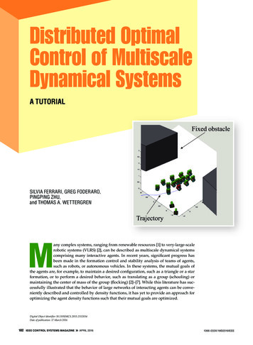
recently developed in [20] based on the generalized reducedgradient (GRG) method. The GRG method belongs to theclass of nested analysis and design numerical methods forsolving PDE-constrained optimization problems [34].The GRG DOC method presented in [20] relies on iteratively solving the forward (14), adjoint (16), and optimalitycriterion (17) as a PDE-constrained minimization problem.Inspired by indirect methods for classical optimal control[23], in the GRG DOC method the microscopic control isparameterized as the sum of linearly independent Fourierbasis functions and then used to obtain approximations ofthe costate and macroscopic state from the solution of theparabolic optimality conditions. Subsequently, holding thecostate and macroscopic-state approximations fixed, themicroscopic control input approximation is updated by agradient-based algorithm that minimizes the augmentedLagrangian function and, ultimately, satisfies the third andfinal optimality condition (17).The adjoint and forward equations are two coupled parabolic PDEs that can be solved efficiently using a modifiedGalerkin method, referred to as CINT [35], which is chosenfor its nondissipative property [36], [37]. In CINT, the PDEsolution is approximated by a linear combination of polynomial basis functions used to satisfy the PDE operatorand Gaussian or radial basis functions used to enforce theboundary conditions at each grid point [35]. Given a control-law parameterization, the forward equation becomes aparabolic PDE with Neumann boundary conditions thatcan be solved numerically to obtain a macroscopic stateapproximation. Once an approximate solution is obtainedfrom the forward equation, the adjoint equation becomes aparabolic PDE in m with Dirichlet boundary conditions,and a numerical solution for m can be obtained by a superposition of polynomial basis and radial basis functions [20].The new and improved control input approximation is thenheld fixed and used to obtain new CINT approximationsfor p and m. This iterative process is repeated until all threeoptimality conditions are satisfied within a user-specifiedtolerance, at which point the algorithm has converged tothe optimal agent distribution p ) .As in classical optimal control, direct DOC methods aretypically easier to implement than indirect methods. Adirect NLP method of solution is reviewed here and analyzed in detail in [18]. The agent PDF p is a conserved quantity that satisfies the Hamilton equations [18]. As a result,the DOC problem can be discretized using a conservativefinite-volume (FV) numerical scheme for representing andevaluating PDEs in algebraic form. This method does notincur dissipative errors associated with coarse-grainedstate discretization, a method that may require reductionin computation [38]. Using the FV approximation, the continuous DOC problem is discretized about a finite set ofcollocation points and then transcribes into a finite-dimensional NLP that can be solved using an efficient mathematical programming algorithm, such as 0500246810 12 14 16x1(a)0p(x, 2108642002468 10 12 14 16p(x, t2)x1(b)Figure 1 An example of a probability density function (PDF) modeled by a six-component Gaussian mixture. (a) An example of aPDF plotted at time t 1 and (b) an example of PDF plotted at time t 2,for a state vector x 6x 1 x 2@T .To discretize the DOC problem, the agent PDF p mustbe parameterized over the solution domain X. As a simpleexample, a finite Gaussian-mixture model is chosen here toprovide this parametric approximation as a superpositionof z components with Gaussian PDFs, denoted by f1, f, fz,and corresponding mixing proportions or weights, denotedby w 1, ., w z . The n-dimensional multivariate Gaussian PDFf j (x i, t) T -11e [- (1/2)(x i - n j) R j (x i - n j)] (19)(2r) n/2 R j 1/2is referred to as the component density of the mixture and ischaracterized by a time-varying mean vector n j ! R n and atime-varying covariance matrix R j ! R n # n with j 1, f, z[39]. Assume that at any t ! (T0, T f ] the optimal agent distribution can be represented asp (x i, t) z/ w j (t) fj (x i, t), (20)j 1where 0 # w j # 1 for all j, / j 1 w j 1, and z is fixed andchosen by the user. Then, an optimal (time-varying) agentdistribution p ) can be obtained by determining the optimal trajectories of the mixture model parameters from theDOC problem. An example of time-varying distributionzapril 2016« IEEE CONTROL SYSTEMS MAGAZINE107
described by a three-component Gaussian mixture with atwo-dimensional state vector x [x 1 x 2] T is shown inFigure 1 at two moments in time t 1 and t 2, where, in thiscase, z 6, and the mixture centers n 1, f, n 6 and weightsw 1, ., w 6 all change over time.The mixture model parameters to be optimized overtime are the weights w j, the elements of n j, and the variances and covariances in R j, with j 1, f, z. In addition tosatisfying the DOC constraints and optimality conditions,the mixture model parameters must be determined suchthat the component densities f1, f, fz are nonnegative andobey the normalization condition for all t ! (T0, T f ] . This isaccomplished by discretizing the continuous DOC problem in state space and time, about a finite set of collocationpoints in X # (T0, T f ] . Let Dt denote a constant discretization time interval and k denote the discrete time index,such that Dt (T f - T0) /K, and thus t k kDt, fork 0, f, K. It is assumed that the microscopic controlinputs, u i, with i 1, f, N, are piecewise constant duringevery time interval, and that the agent distribution at timet k can be represented byp k p (x i, t k) z/ w j (t k) fj (x, t k)j 1z/T -11e [- (1/2)(x i - n jk) R jk (x i - n jk)] .(2r) n/2 R jk 1/2/ w jkj 1 (21)The set of weights {w jk} and the elements of n jk and R jk, forall j, k, are grouped into a vector that represents the trajectories of the mixture model parameters in discrete time.The FV approach partitions the state-space X into FVsdefined by a constant discretization interval Dx ! R n thatare each centered about a collocation point x l ! X 1 R n,with l 1, ., L [38]. Let p l, k and u l, k denote the finite-difference approximations of p (x l, t k) and c [p (x l, t k)], respectively.Then, the finite-difference approximation of the advectionequation is obtained by applying the divergence theoremto (14) for every FV such that p k 1 p k Dtt k, wheretk -#S [p k f (p l,k, u l,k, t k)] nt dS, (22)and S and nt denote the FV boundary and unit normal,respectively.Now, letting Dx (j) denote the jth element of D x, the discretized DOC problem can be written as the finite-dimensional NLPmin J D nLKj 1l 1k 1/ Dx (j) / [z l,K Dt / L (p l,k, u l,k, t k)],subject to p k 1 - p k - Dtt k 0, k 1, f, K,nLj 1l 1/ Dx (j) / p l,k - 1 0, k 1, f, K,p l, 0 p 0 (x l), x l ! X,p l, k 0, x l ! 2X, k 1, f, K, (23)where z l, K z (p l, K) is the terminal constraint. The solution) of the above NLP can be obtained using an SQP algo108 IEEE CONTROL SYSTEMS MAGAZINE»april 2016rithm that solves the KKT optimality conditions by representing (23) as a sequence of unconstrained quadraticprogramming subproblems [40]. The reader is referred to[18] for a detailed description and analysis of the abovedirect DOC method, including the computational complexity analysis and comparison with classical direct optimalcontrol methods.Distributed Optimal Control Feedback Control LawAlthough the optimal agent control laws are obtainedtogether with the optimal agent PDF, it is often more usefulin practice to separate the planning and control designssuch that state measurements can be fed back and accountedfor by the agent while attempting to realize or “track” theoptimal time-varying PDF p ) . By this approach, the actualagent PDF can be estimated and considered by the feedback control law, and the feedback control can be designedto achieve additional local constraints or account for communication constraints. Various techniques, including Voronoi diagrams, Delaunay triangulations, and potentialfield methods, have been
qx[(tt),u() ,]t # 0 d#1. (3) When random effects can be neglected, optimal control problems in the form (1)-(3) can be approached by solving the necessary conditions for optimality known as Euler- Lagrange equations, which may be derived using calculus of variations [21]. Another approach is to use the recurrence