WIXLIB

520A. KUMAR AND A. VLADIMIRSKY(A3) For every x Ω, the scaled vectogramV (x) {f(x, a)/K(x, a) a A}is a strictly convex set, containing the origin in its interior.The key idea of dynamic programming is to introduce the value function u(x), describingthe minimum cost needed to exit Ω starting from x:u(x) inf J (x, a(·)).a(·) A(2.3)Bellman’s optimality principle [6] shows that, for every sufficiently small τ 0, Z τ u(x) infK(y(t), a(t)) dt u(y(τ )) ,a(·) 0(2.4)where y(·) is a trajectory corresponding to a chosen control a(·). If u(x) is smooth, a Taylorexpansion of the above formula can be used to formally show that u is the solution of a staticHamilton-Jacobi-Bellman PDE:min {K(x, a) u(x) · f (x, a)} 0,a Au(x) q(x),for x Ω;for x Ω.(2.5)Unfortunately, a smooth solution to Eqn. 2.5 might not exist even for smooth f ,K, q, and Ω.Generally, this equation has infinitely many weak Lipschitz-continuous solutions, but the uniqueviscosity solution can be defined using additional conditions on smooth test functions [11, 12].It is a classic result that the viscosity solution of this PDE coincides with the value function ofthe above control problem.Under the above assumptions the value function u(x) is locally Lipschitz-continuous on Ω,an optimal control a(·) actually exists for every x Ω (i.e., min can be used instead of inf informula 2.3), and the minimizing control value a (in equation 2.5) is unique wherever u(x)is defined [1]. The characteristic curves of this PDE are the optimal trajectories of the controlproblem. The points where u is undefined are precisely those, where multiple characteristicsintersect (or, alternatively, the points for which multiple optimal trajectories are available). Wewill let Γ be a set of all such points. By Rademacher’s theorem, Γ has a measure zero in Ω̄.We note that the assumptions (A2-A3) can be relaxed at the cost of additional technicaldetails. For example, if V (x) is not convex, the existence of an optimal control is not guaranteedeven though the value function can still be recovered from the PDE (2.5) and there existsuboptimal controls whose cost is arbitrarily close to u(x). On the other hand, if V (x) doesnot contain the origin in its interior, then the reachable set R x Ω there exists a control leading from x to Ω in finite timeneed not be the entire Ω. In that case, R is a free boundary. We refer readers to [1] for furtherdetails.The above framework is also flexible enough to describe the task of optimally reaching somecompact target T Ω without leaving Ω. To do that, we can simply pose the problem on anew domain Ωnew Ω\T , defining the new exit cost q new to be infinite on Ω and finite on

521An Efficient Method for Multiobjective Optimal Control T . The assumptions (A0-A3) guarantee the continuity of the value function on Ω even in thepresence of state-constraints; k1 0 and the fact that the origin is in the interior of V (x) yieldboth Soner’s “inward pointing” condition along the boundary of the constraint set (as in [36])and the local controllability (as in [2], for example).Remark 2.1. The continuity of u on Ω̄ is a more subtle issue requiring additional compatibilityconditions on q even if that function is continuous; otherwise, the boundary conditions aresatisfied by the value function “in viscosity sense” only [1]. However, due to our very strongcontrollability assumption (A3), the local Lipschitz-continuity of u in the interior is easy toshow even if q is discontinuous, as allowed by (A0). Without assumption (A3) or its equivalent,discontinuous boundary data typically leads to discontinuities in the value function in theinterior as well. Such is the case for the augmented PDE defined in section 3.3.Before continuing with the general case we consider two particularly useful subclasses ofproblems.Geometric dynamics. Suppose A {a Rn a 1} and, for all x Ω, a A\{0},K(x, a) a K(x, a/ a ),f (x, a) f (x, a/ a )a,and f (x, 0) 0.Then it is easy to show that the cost of any trajectory is reduced by traversing it as quicklyas possible; i.e., we can redefine A Sn 1 {a Rn a 1} without affecting the valuefunction. In that case, the control value a is simply our choice for the direction of motion andf is the speed of motion in that direction. The equation (2.5) now becomesmin {K(x, a) ( u(x) · a) f (x, a)} 0.a Sn 1(2.6)A further simplification is possible if the speed and cost are isotropic, i.e., f (x, a) f (x) andK(x, a) K(x). In this case, the minimizing control value is a u(x)/ u(x) and (2.5)reduces to an Eikonal PDE: u(x) f (x) K(x).(2.7)The characteristics of the Eikonal equation coincide with the gradient lines of its viscosity solution. That special property can be used to construct particularly efficient numerical methodsfor this PDE; see section 2.4.Time-optimal control. If K(x, a) 1 for all x and a, then J (x, a(·)) Tx,a q(y(Tx,a )).Interpreting q as an exit time penalty, we can restate this as a problem of finding a time-optimalcontrol starting from x. The PDE (2.5) becomesmax { u(x) · f (x, a)} 1.a A(2.8)We note that the value function for every exit-time optimal control problem satisfying assumptions (A0-A3) can be reduced to this time-optimal control case by setting K new 1 andf new (x, a) f (x, a)/K(x, a); a proof of this for the case of geometric dynamics can be foundin [41].A combination of these two special cases is attained when K 1 and f 1, leading to aPDE u(x) 1. If the boundary condition is q 0, then u(x) is simply the distance from xto Ω.

522A. KUMAR AND A. VLADIMIRSKY2.2. Semi-Lagrangian discretizationsSuppose X is a grid or a mesh on the domain Ω̄ and for simplicity assume that Ω iswell-discretized by X. We will use M X to denote the total number of meshpoints in X.A natural first-order accurate semi-Lagrangian discretization of equation (2.5) is obtained byassuming that the control value is held fixed for some small time τ . If U (x) is the approximationof the value function at the mesh point x X, then the optimality principle yields the followingsystem:U (x) min {τ K(x, a) U (x τ f (x, a))} ,a AU (x) q(x), x X. x X\ Ω;(2.9)Since x̃a x τ f (x, a) usually is not a gridpoint, a first-order accurate reconstruction isneeded to approximate U (x̃) based on values of U at nearby meshpoints1) . Discretizations ofthis type were introduced by Falcone for time-discounted infinite-horizon problems, which canbe related to the above exit-time problem using the Kruzhkov transform [16, 17].In case of geometric dynamics, another natural discretization is based on the assumptionthat the direction of motion is held constant until reaching a boundary of a simplex. Fornotational simplicity, suppose that n 2 and S(x) is the set of all triangles in X with a vertexat x. For every s S(x), denote its other vertices as xs1 and xs2 . Suppose x̃a x τa f (x, a)alies on the segment xs1 xs2 . Let Ξ ξ (ξ1 , ξ2 ) ξ1 ξ2 1 and ξ1 , ξ2 0 .Then x̃a ξ1 xs1 ξ2 xs2 for some ξ Ξ and U (x̃a ) ξ1 U (xs1 ) ξ2 U (xs2 ). Alternatively,given x̃ξ ξ1 xs1 ξ2 xs2 , we can defineaξ (x̃ξ x)/ x̃ξ x and τξ x̃ξ x /f (x, aξ ).This yields the following system of discretized equations:U (x) min min {τξ K(x, aξ ) (ξ1 U (xs1 ) ξ2 U (xs2 ))} ,s S(x) ξ ΞU (x) q(x), x X. x X\ Ω;(2.10)Discretizations of this type were used by Gonzales and Rofman in [18]. Both discretizations(2.9) and (2.10) were also earlier derived by Kushner and Dupuis approximating continuousoptimal control by controlled Markov processes [23]. In the appendix of [35] we demonstratedthat (2.10) is also equivalent to a first-order upwind finite difference approximation on thesame mesh X.2.3. Causality, dimensionality & computational efficiencyWe note that both of the above discretizations result in a system of M non-linear coupledequations. Finding a numerical solution to that system efficiently is an important practicalproblem in itself.1) If x is close to Ω, it is possible that x̃ 6 Ω̄. This can be handled by either enlarging X to cover someaneighborhood of Ω (see, e.g., [4]) or by decreasing τ in such cases to make x̃a Ω. The latter strategy is alsoadopted in our implementation of the method in section 3.4.

An Efficient Method for Multiobjective Optimal Control523Suppose all meshpoints in X are ordered x1 , . . . , xM and U (U1 , . . . , UM ) is a vector ofcorresponding approximate values. The above discretized equations can be formally written asU F (U ) and one simple approach is to recover U by fixed-point iterations, i.e., U k 1 F (U k ),where U 0 is an appropriate initial guess for U . This procedure is generally quite inefficient sinceeach iteration has a O(M ) computational cost and a number of iterations needed is at leastO(M 1/n ).A Gauss-Seidel relaxation of the above is a typical practical modification, where the entries of U k 1 are computed sequentially and the new values are used as soon as they becomek 1kavailable: Uik 1 Fi (U1k 1 , . . . , Ui 1, Uik , . . . , UM). The number of iterations required to converge will now heavily depend on the PDE, the particular discretization and the ordering of themeshpoints. We will say that a discretization is causal if there exists an ordering of meshpointssuch that the convergence is attained after a single Gauss-Seidel iteration. For example, if thedynamics of the control problem is such that one of the state components (say, y1 ) is monotoneincreasing along any feasible trajectory y(t), then ordering all the meshpoints in ascendingorder by x1 would guarantee that only one Gauss-Seidel iteration is needed. Such ordering isanalogous to a simple time-marching (from the past into the future) used with discretizationsof time-dependent PDEs (e.g., in recovering the value function for fixed-horizon optimal controlproblems). If a causal ordering is explicitly known a priori (as in the above example), we referto such discretizations as explicitly causal.Explicit causality is a desirable property since it results in computational efficiency. Supposeu(x) is a viscosity solution of some boundary value problem. Historically, two approaches havesought to capitalize on explicit causality in solving more general static PDEs. First, it is oftenpossible to formulate a different time-dependent PDE on the same domain Ω so that its viscositysolution φ is related to u as follows:u(x) t φ(x, t) 0.The PDE for φ is then solved by explicit time-marching; moreover, since only the zero level setof φ is relevant for approximating u, the Level Set Methods are applicable e.g., see [27,30]. Asidefrom increasing the dimensionality of the computational domain, this approach is also subjectto additional CFL-type stability conditions, which often impact the efficiency substantially.Alternatively, in some applications (e.g., seismic imaging) a “paraxial” approximation resultsfrom assuming that all optimal trajectories must be monotone in one of the state components(say, y1 ) even if the same is not true for all feasible trajectories. This leads to a time-likemarching in x1 direction (essentially solving a time-dependent PDE on an (n 1)-dimensionaldomain); see, e.g., [28]. This method is certainly computationally efficient, but if the assumptionon monotonicity of optimal trajectories is incorrect, it does not converge to the solution of theoriginal PDE.2.4. Efficient methods for non-explicitly causal problemsFinding the right ordering without increasing the dimensionality has been the subject ofmuch work in the last fifteen years. This task can be challenging for discretizations which arecausal, but not explicitly causal.For the isotropic control problems and the Eikonal PDE (2.7), an equivalent of discretization (2.10) on a Cartesian grid is monotone-causal in the sense that Ui cannot depend on Ujif Uj Ui . This makes it possible to find the correct ordering of gridpoints (ascending in U )

524A. KUMAR AND A. VLADIMIRSKYat run-time, effectively de-coupling the system of discretized equations. This idea, the basis ofDijkstra’s classic method for shortest paths on graphs [14], yields the computational complexityof O(M log M ). Tsitsiklis has introduced the first Dijkstra-like algorithm for semi-Lagrangiandiscretization on a Cartesian grid in [40]. A Dijkstra-like Fast Marching Method was introducedby Sethian for Eulerian upwind finite-difference discretizations of isotropic front propagationproblems [29]. The method was later extended by Sethian and collaborators to higher-orderaccurate discretizations on grids and unstructured meshes, in Rn and on manifolds, and to related non-Eikonal PDEs; see [30], [33], and references therein. For anisotropic control problems,the discretization (2.10) generally is not causal, but the computational stencil can be expandeddynamically to regain the causality. This is the basis of Ordered Upwind Methods [34, 35, 41],whose computational complexity is O(ΥM log M ), where Υ measures the amount of anisotropypresent in the problem.The idea of alternating the directions of Gauss-Seidel sweeps to “guess” the correct meshpoint ordering was employed by Boue and Dupuis to speed up the convergence in [7]. ForEulerian discretizations of HJB PDEs, the same technique was later used as a basis of FastSweeping Methods by Tsai, Cheng, Osher, and Zhao [39, 43]. Even though a finite number ofGauss-Seidel sweeps is required in the Eikonal case, resulting in a computational cost of O(M ),the actual number of sweeps is proportional to the maximum number of times an optimaltrajectory may be changing direction from quadrant to quadrant. A computational comparisonof fast marching and fast sweeping approaches to Eikonal PDEs can be found in [19, 20].3. Multi-criterion Optimal ControlUnlike the classical case considered in section 2, in realistic applications there is often morethan one criterion for optimality. For a system controlled in Ω Rn , there may be a numberof different running costs K0 , . . . , Kr and a number of different terminal costs q0 , . . . , qr (allof them satisfying assumptions (A0-A3)) resulting in (r 1) different definitions J0 , . . . , Jr ofthe total cost for a particular control. A common practical problem is to find a control a (·)minimizing J0 (x, a (·)) but subject to constraints Ji (x, a (·)) Bi for all i 1, . . . , r.We will refer to a control minimizing J0 without any regard to constraints as primaryoptimal. A control minimizing some Jj (for j 0) without any regard to other constraints willbe called j-optimal (or simply secondary-optimal, when j is clear from the context). A controlminimizing J0 subject to all of the above constraints on Ji ’s will be called constrained-optimal.For a fixed x Ω, we will say that a control a1 (·) is j-dominated by a control a2 (·) ifJi (x, a2 (·)) Ji (x, a1 (·)) for all i 0, . . . , r and Jj (x, a2 (·)) Jj (x, a1 (·)). We will alsosay that a1 (·) is dominated by a2 (·) if it is j-dominated for some j {0, . . . , r}. E.g., theconstrained-optimal control a (·) described above might be dominated, but will not be 0dominated by any control. Any control a (·) dominating a (·) will have the same primarycost J0 and will also satisfy the same constraints; moreover, it will even spend less in at leastone of the secondary costs J1 , . . . , Jr .We will say that a(·) is Pareto-optimal for x, if it is not dominated by any other control.In that case, its vector of costs corresponds to a point on a Pareto-front P(x) in a J0 , . . . , Jrspace; see Figure 3.2A.Our goal is to find an efficient numerical method for approximating the costs associatedwith Pareto-optimal controls. The efficiency requires solving this problem for all x Ω simultaneously.

525An Efficient Method for Multiobjective Optimal ControlWe begin by showing how to compute the total cost Ji incurred by using a control optimalwith respect to a different running cost (section 3.1). We then describe a recent method dueto Mitchell and Sastry for recovering a convex portion of the Pareto front by scalarization(section 3.2). Finally, in section 3.3 we describe a new method for solving fully this problem byaugmenting the system state to include the “budget remaining” in each secondary cost.3.1. Total cost along “otherwise optimal” trajectoriesWe will use ui (x) to denote the value function with respect to Ji if all other costs areignored. As explained in section 2.1, ui (x) can be recovered as a viscosity solution of thePDE (2.5), if we set K Ki and q qi .Given a different value function u derived for some other cost J , we will define a restrictedset of J -optimal controls Au,x a(·) A J (x, a(·)) u(x) .As explained in section 2.1, if J satisfies the assumptions (A0-A3), then Au,x will be non-emptyfor every x Ω and will contain a single element for every x Ω\Γ.We will use vi (x) to denote a J -optimality-restricted value function with respect to Ji :vi (x) infJi (x, a(·)).a(·) Au,x(3.1)This notation relies on a fixed choice of J and u, and we will specify J explicitly in each caseto avoid ambiguity. For the cases when J Jj and u uj , we will use vij instead of vi .According to this definition, we also have vii ui .The following properties of Pareto fronts follow from the above definitions. The proofs aresimple and we omit them for the sake of brevity.Property 3.1. vi (x) ui (x) for x Ω̄ and for any choice of J satisfying assumptions(A0 A3).Property 3.2. Suppose u(x) is the value function corresponding to some J that satisfies assumptions (A0 A3). If Ki and qi also satisfy (A0 A2), then vi (x) is lower semi-continuouson Ω and continuous wherever u(x) is differentiable. Property 3.3. Let U(x) (J0 , . . . , Jr ) Rr 1 Ji uj (x), j 0, . . . , r . Then for anyx Ω̄, we have1. P(x) U(x) and2. (vi0 (x), . . . , vir (x)) P(x) for all i 0, . . . , r.Property 3.4. If r 1, then P(x) [v00 (x), v01 (x)] [v11 (x), v10 (x)].Suppose u is a smooth solution to the PDE (2.5). Then Γ and for every x Ω thereexists a unique optimal/minimizing control value a a (x, u(x)) A. The local rate ofincrease of Ji along the corresponding trajectory is Ki (x, a ). This yields a system of (r 1)linear PDEs vi (x) · f (x, a ) Ki (x, a ), x Ω;vi (x) qi (x), x Ω;i 0, . . . , r.(3.2)

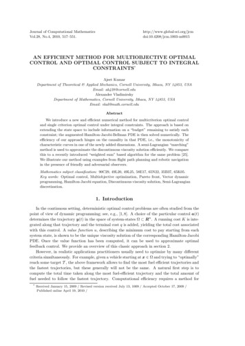
526A. KUMAR AND A. VLADIMIRSKYu0x0u110v1,0x0x1v0,110x1Fig. 3.1. Cost along “otherwise optimal” trajectories. A simple one-dimensional example: Ω̄ [0, 1],f K0 K1 1, and q0 (0) q1 (0) q1 (1) 0, but q0 (1) 0.4. Similar discontinuities may occureven if q0 q1 (when K0 6 K1 ).This system is coupled to a nonlinear equation (2.5), since a is generally not available apriori unless u is already known.In the Eikonal case (when A Sn 1 , f (x, a) f (x)a and K(x, a) K(x)), the optimaldirection of motion isf (x) u(x)a u(x), u(x) K(x)and the system (3.2) can be rewritten as vi (x) · u(x) Ki (x, a )K(x)/f 2 (x), x Ω; x Ω;vi (x) qi (x),i 0, . . . , r.(3.3)If u is not smooth, the functions vi may become discontinuous (see Figure 3.1) and ageneralized solution is needed to define vi (x) at any points x Γ. Luckily, Bellman’s optimalityprinciple provides an alternative definition to resolve this ambiguity:vi (x) limτ 0 min {τ K(x, a ) vi (x τ f (x, a )) } ,a Au,xwhere Au,x A is the set of minimizing control values in (2.5). If x 6 Γ, then the Au,x consistsof a single element and this formulation is equivalent to (3.2). Whether or not a is unique,the above formula yields the lower semi-continuity of vi . It can also be used (with a fixed smallτ 0) to derive a first-order semi-Lagrangian discretization of (3.2).We note that the key technical idea employed above (solving a linear equation along thecharacteristics of another PDE) is well-known and useful in many applications. A commonversio

2. Single-criterion Dynamic Programming 2.1. Exit-time optimal control To begin, we consider a general deterministic exit-time optimal control problem. This is n is an Suppose A Rm is a compact set of control values, and the set of admissible controls A consists of all measurable fun