Transcription
1514IEEE TRANSACTIONS ON AUTOMATIC CONTROL, VOL. 46, NO. 10, OCTOBER 2001A Canonical Correlations Approach to MultiscaleStochastic RealizationWilliam W. Irving and Alan S. Willsky, Fellow, IEEEAbstract—We develop a realization theory for a class of multiscale stochastic processes having white-noise driven, scale-recursive dynamics that are indexed by the nodes of a tree. Given thecorrelation structure of a 1-D or 2-D random process, our methodsprovide a systematic way to realize the given correlation as thefinest scale of a multiscale process. Motivated by Akaike’s use ofcanonical correlation analysis to develop both exact and reducedorder model for time-series, we too harness this tool to developmultiscale models. We apply our realization scheme to build reduced-order multiscale models for two applications, namely linearleast-squares estimation and generation of random-field samplepaths. For the numerical examples considered, least-squares estimates are obtained having nearly optimal mean-square errors,even with multiscale models of low order. Although both field estimates and field sample paths exhibit a visually distracting blockiness, this blockiness is not an important issue in many applications.For such applications, our approach to multiscale stochastic realization holds promise as a valuable, general tool.Index Terms—Least squares methods, realization theory, simulation, singular value decomposition, stochastic processes.I. INTRODUCTIONN THIS PAPER, we exploit well-established controlconcepts to develop a realization theory for the classof multiscale stochastic processes introduced in [4], [5].These processes have white-noise driven, scale-recursivedynamics, directly analogous to the time-recursive dynamicsof Gauss-Markov time-series models. Experimental and theoretical results have demonstrated that this class of processesis quite rich statistically; the self-similarity of fractionalBrownian motion can be represented [5], as can any given 1-Dwide-sense (WS) reciprocal process or 2-D Markov randomfield (WSMRF) [18].1 Complementing this statistical richnessare the efficient image processing algorithms to which multiscale models lead. For example, a scale-recursive algorithmhas been developed that directly generalizes the Kalmanfilter and related Rauch–Tung–Striebel (RTS) smoother [5].IManuscript received December 2, 1996; revised April 29, 1997, February 20,1998, and November 27, 2000. Recommended by Associate Editor J. Spall. Thiswork was supported by the Air Force Office of Scientific Research, under GrantAFOSR-F496-20-93-1-0604 and the Army Research Office under Grant ARODAAL03-92-G-0015.W. W. Irving is with Fidelity Investments, Merrimack, NH 03054 USA(e-mail: William.Irving@FMR.COM).A. S. Willsky is with the Department of Electrical Engineering and Computer Science, the Massachusetts Institute of Technology (MIT), Cambridge,MA 02139 USA (e-mail: willsky@mit.edu).Publisher Item Identifier S 0018-9286(01)09591-5.1Thedefinition and properties of wide-sense reciprocal processes andWSMRFs are nicely summarized in [8].This algorithm incorporates noisy measurements of a givenmultiscale process to calculate both smoothed estimates andassociated error covariances. Another algorithm has beendeveloped for likelihood calculation [17]. In contrast to traditional 2-D optimal estimation formulations based on Markovrandom fields, which lead to iterative algorithms having aper-pixel computational complexity that typically grows withimage size, these multiscale algorithms are noniterative andhave a per-pixel complexity independent of image size [18],[19]. Substantial computational savings can thus result, asevidenced by exploitation of the multiscale framework in manyapplications, including computer vision (e.g., calculation ofoptical flow [19]), remote sensing (e.g., optimal interpolationof sea level variations in the North Pacific Ocean from satellitemeasurements, treating the ocean as either static [11], or morerecently as dynamic [12]) and geophysics (e.g., characterizingspatial variations in hydraulic conductivity from both point andnonlocal measurements [6]).In exactly the same way that Kalman filtering requires theprior specification of a state-space model before least-squareestimation or likelihood calculation can be carried out, so doesmultiscale statistical processing require such prior modeling.The techniques developed in this paper provide the neededmodeling tools: given the correlation structure of a 1-D or2-D random process,2 these tools can be used to realize thecorrelation as the finest of a multiscale process. Because thereis typically a conflict between model complexity and accuracy,we mainly focus on the case where a constraint is imposed onthe allowed model state dimension; the objective then is to builda model whose finest-scale correlation structure best matchesthe desired correlation, subject to the dimension constraint.Our focus on realizing finest-scale statistics is motivated bythe not insignificant class of applications in which the finestscale is really the only one of interest. For instance, in manyimage-processing applications (such as de-noising problems[15], or terrain segmentation [17]), the finest-scale process is apixel-by-pixel representation of the image, the measurementsare noisy observations of some subset of the pixels, and theobjective is either to estimate the value of each image pixel[15] or to calculate the likelihood of the observations [17].Similarly, in distributed parameter estimation problems (suchas those arising in remote sensing [12] or geophysics [6]), thefinest-scale process is a sampled version of the parameter ofinterest (e.g., hydraulic conductivity [6]), the measurements arenoisy observations related to the parameter, and the objective2The terminology 1-D, 2-D, or multidimensional random process is used hereto indicate that the dimension of the independent variable of the process is 1-D,2-D, or multidimensional.0018–9286/01 10.00 2001 IEEE
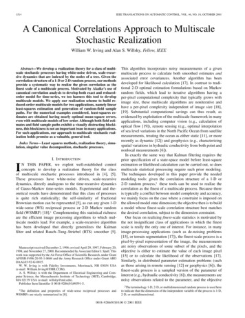
IRVING AND WILLSKY: A CANONICAL CORRELATIONS APPROACH TO MULTISCALE STOCHASTIC REALIZATIONis to estimate the parameter. For all of these problems, themultiscale framework provides an efficient statistical approachfor obtaining estimates and error covariances or calculatinglikelihoods, even though every other aspect of these problemsinvolves only the finest scale.Our approach to multiscale stochastic realization takes advantage of the close relationship the problem shares with its moretraditional, time-series counterpart. To clarify this relationship,we first observe that each node in a -th order tree has childrenand a single parent, and hence partitions the remaining nodessubtrees, one associated with each of these child andintoparent nodes. (A second-order tree, which is often used to indexmultiscale representations of time series, is illustrated in Fig. 1.)Related to this partitioning property is the Markov property thatis the value of the state atmultiscale processes possess: ifthe states in the correspondingnode , then conditioned onsubtrees of nodes extending away from are uncorrelated [18]. The connection to the time-series realization problemis that in both contexts, the role of state information is to providean information interface among subsets of the process. This interface must store just enough process information to make thecorresponding process subsets conditionally uncorrelated. Thekey challenge is that while in the time-series case this interfaceis between two subsets of the process (i.e., the past and the future), in the multiscale case, the interface is among multiple (i.e.,) subsets of the process.We exploit the connection between the time-series and multiscale realization problems by adapting to the multiscale context work done in [1] and [2] on reduced-order time-series modeling. The work in [1] and [2] addresses two issues. First, forexact realizations, a method is devised for finding the minimaldimension and corresponding information content of the state.Second, for reduced-order, approximate realizations, a methodis devised for measuring the relative importance of the components of the information interface provided by the state, so thata decision can be made about which components to discard ina reduced-order realization. The latter is accomplished using aclassical tool from multivariate statistics, namely canonical correlation analysis [13]. We decompose our multiscale problemprocess subsets into a collecof decorrelating jointlytion of problems of decorrelating pairs of process subsets.We then demonstrate that with respect to a particular decorrelation metric, canonical correlation analysis can in principlebe used to solve optimally each of the pairwise decorrelationproblems. Furthermore, these pairwise solutions can be concatenated to yield a sub-optimal solution to the multi-way decorrelation problem. The solution to this decorrelation problem leadsreadily to values for all the multiscale model parameters.We apply our realization scheme to build reduced-order multiscale models for two applications, namely linear least-squaresestimation and generation of random-field sample paths. For thenumerical examples considered, we obtain least-squares estimates having mean-square errors that are nearly optimal, evenwith multiscale models of very low order. Although both fieldestimates and field sample paths exhibit a visually distractingblockiness, this blockiness is not really an issue in many applications. For such applications, our approach to multiscale realization holds promise as a valuable, general tool.1515Fig. 1. The first four levels of a second-order tree are shown. The parent ofand s .node s is denoted by s and the two offspring are denoted by sThe random vectors and contain, respectively, the finest-scale stateinformation that does and does not descend from the node s.The remainder of this paper is organized in the following way.In Section II, the multiscale framework is more formally introduced, and a measure of decorrelation is defined. In Section III,the modeling problem is precisely formulated, and a solution ispresented for the case that full-order, exact models are sought.Then, in Section IV, the solution to the modeling problem is presented for the more challenging case that reduced-order, approximate models are sought. In Section V, two numerical examplesare presented, and finally in Section VI, a summary is provided.Details of the proofs are relegated to Appendices A–C at the endof the paper.II. PRELIMINARIESA. State-Space Models on th-Order TreesThe models introduced in [4], [5], [19] describe multiscalestochastic processes indexed by nodes on a tree. A th-ordertree is a pyramidal structure of nodes connected such that eachnode (other than the leaf nodes) has offspring nodes. We, whereassociate with each node a vector-valued statestate vectors at the th level of the treein general, the) can be interpreted as information about(forthe -th scale of the process. In keeping with the conventionsestablished in [4], [5], we define an upward (fine-to-coarse)is the parent of node , and ashift operator such thatcorresponding set of downward (coarse-to-fine) shift operators, such that the offspring of node are. Fig. 1 depicts an example of thegiven by,in a second-order tree.relative locations of , , andThe dynamics implicitly providing a statistical characterizahave the form of an autoregression in scaletion of(1), with aThis regression is initialized at the root node,having mean zero and covariance. Thestate variablerepresents white driving noise, uncorrelated acrosstermscale and space, and also uncorrelated with the initial condition; this noise is assumed to have mean zero and covariance. Sinceandare zero-mean, it follows that
1516IEEE TRANSACTIONS ON AUTOMATIC CONTROL, VOL. 46, NO. 10, OCTOBER 2001is a zero-mean random process.3 Furthermore, since the drivingis white, the correlation structure of the processnoiseis characterized completely byand the auto-regression paandfor all nodes.rametersThe statistical structure of multiscale processes can be exploited to yield an extremely efficient algorithm for estimating, based upon noisy observations. These observationstake the formwhere the noiseis white, has covariance, and is unat all nodes on the tree. Just like the Kalmancorrelated withfilter and the RTS smoother, this estimation algorithm has a recursive structure, and yields both state estimates and associatederror covariances. For a multiscale process having states of dimension and indexed on a tree with nodes, the number of. Thus, the algorithm is quiterequired computations isefficient, particularly when the dimension of the state vectors islow.B. Markov Property of Multiscale ProcessesMultiscale processes possess an important Markov property,. To describe thestemming directly from the whiteness ofform of this property of interest to us, we associate with each treecontains all of the finest-scale nodesnode a set , wherethat descend from . We also associate with each node the. The random vector contains therandom vectors and, stacked into a vector, whileelements of the setcontains the elements of the complementary set, stacked into a vector. These conventionsare illustrated in Fig. 1. It will sometimes prove convenient toby; we freely use both forms. To relatedenoteand, we introduce the matrix, whereis the, and is a nodelinear least-squares estimate of , givenor represents a set of nodes.The Markov property, as it relates explicitly to the finest scale,can now be stated as follows [7]:.We use this property to relate the dimension ofrelation among the vectorsend, (2) and (3) together imply thatrankdimensionIf the finest-scale covariancemust match exactly someprespecified covariance, then this proposition provides a lowerbound on the required multiscale state dimension. In the ratherlikely case that the involved cross-covariance matrices have fullrank, this dimension constraint becomes quite stringent. Thus,to keep the multiscale estimation algorithm computationally efficient, we find considerable motivation to turn to reduced-order(approximate) realizations.C. The Generalized Correlation CoefficientFor the purposes of developing reduced-order models, it willprove convenient to have a scalar measure of the correlationamong a collection of random vectors. We thus introduce aso-called generalized correlation coefficient. In keeping withstandard conventions, we define as follows the correlation cobetween two scalar valued random variablesefficientand :iffor(5)otherwise.Then, for a pair of vector-valued random variableswe define their generalized correlation coefficientand,bywhere the dummy argument (for) is a column vectorhaving the same dimension as . Finally, we extend the definito a collection of random vectors,tion ofin the following way:(2)Each of these correlation coefficients has a conditioned version. To define them, we first let random vector contain the, whereconditioning information. Also, we letis(here and elsewhere) we adhere to the convention thatthe linear least-squares estimate of given . Finally, we define(3)(6)withuncorrelatedcross-covariance of random vectors and ). By elementarylinear algebra [22], the rank of the cross-covariance in (4) is, which in turn is upperupper-bounded by the rank of. The following propositionbounded by the dimension ofthus follows.Proposition 1:to the cor. Toward this(4)(Here and elsewhere, we adhere to the notational conventionis the covariance of random vector andis thethat3The mean of x(1) can be set to any arbitrary value, by suitably adjusting themean of x(0) and w (1).III. FORMULATION AND INITIAL INVESTIGATIONREALIZATION PROBLEMOFThe realization problem of interest in this paper is to builda multiscale model, indexed on a given tree structure, to realize some prespecified, finest-scale covariance. We begin withanda random vector , having the prespecified covariancehaving an established correspondence with the finest scale of thegiven tree. For example, might be a random field (written for
IRVING AND WILLSKY: A CANONICAL CORRELATIONS APPROACH TO MULTISCALE STOCHASTIC REALIZATIONsimplicity as a vector), with the finest scale of the tree (e.g., aquadtree) being a pixel-by-pixel representation of the field. Our,objective is to specify values for the model parametersand, to achieve the best match possible between theand the desired covariance.actual, realized covarianceIn making the specification, we impose on each node a dimension constraintdimension(7)With the dimension constraint imposed, Proposition 1 showsthat it may not be possible to achieve strict equality betweenand, thus justifying our distinct notation for each. Forand.convenience, we also introduce the random vectorsas andThese are defined to have the same relation tohave to . To be more precise, suppose that the th componentmaps to theth (th) component of ; then,ofmaps to theth (th)the th component ofhas the same dimension ascomponent of , where. It will sometimes prove convenient to denoteby; we freely use both forms.A. Full-Order RealizationsWhen the dimension constraint is discarded, the realizationproblem becomes conceptually simpler and exact realizations) become possible. We(i.e., realizations for whichbegin by analyzing this case.A notable class of multiscale processes in the context of exactis a linearrealizations is those in which each state variablefunction of the finest-scale process1517Comparing (1) and (10), and using standard results from linearleast-squares estimation, the model parameters can be seen tosatisfy the following relations:(11a)(11b)andFinally, again using (8) and the facts that, the covariances appearing in (11a) and (11b)can be expressed as simple functions of the internal matricesand the finest-scale covariance(12a)(12b)A natural question at this point is how to devise the internalmatrices for an extact, internal realization of a given finest-scalecovariance. At the finest-scale nodes, the internal matrices areeasy to determine; they are implicitly defined by the association between finest-scale nodes and the components of . Foris assigned to a disexample, if each scalar component offor each finest-scaletinct finest-scale node, then clearlynode. At any coarse-scale node (i.e., any nodes above the finestscale), a necessary condition for (2) and (3) to hold in an exact,fulfill the following decorrelating role:internal model is that(13)The necessity of (13) can be justified in the following manner:(8)obeying this relationship can clearly be seenA state vectorto represent an aggregate (coarse) description of the finest-scaleassociprocess descending from . We refer to the matrixated with node as the node’s internal matrix, and we refer toas internal realizamultiscale processes for which (8) holdstions. The notion of internal stochastic realizations is standardin time-series analysis [16], [20], with our use of the conceptrepresenting a natural adaptation.Our interest in internal realizations stems from the conve,, andcannient fact that the model parametersbe specified completely in terms of the internal matrices andthe finest-scale covariance. In other words, once values valuesfor the internal matrices have been determined, values for the,andfollow easily. To seemodel parametersintothis fact, we begin by substituting (8) evaluated atand using the fact thattoyield(9)andcan then be computed by notingThe parametersthat (1) represents the linear least-squares prediction ofbased upon, plus the associated prediction error(10)Here, the first equality follows from the facts that the realization is exact and internal, the second equality follows from theand the conditional generalized correlationdefinitions ofcoefficient, and the final equality follows from (2) and (3).As we now show, (13) is not only necessary for an exact,internal realization, but is also sufficient for building an exactrealization.matricesProposition 2: Suppose that for all nodes , the,,satisfy (13), and that the multiscale system matricesare defined in terms of thematrices via (9) andand(14a)(14b)Then, for any nodes)andat the same scale (possibly with(15)A proof of Proposition 2 is contained in Appendix A. The following special case of the proposition is of particular interest.Corollary 1: If the conditions in Proposition 2 hold, then.Proof: For any and at the finest scale, the internal maandare identity matrices, and hence (15) impliestrices. But also, by definition,that
1518IEEE TRANSACTIONS ON AUTOMATIC CONTROL, VOL. 46, NO. 10, OCTOBER 2001. Thus,, and the corollary immediately follows.QEDTo summarize, there is a three-stage procedure for realizingexactly any desired finest-scale covariance: (i) establish a correspondence between finest-scale nodes and components of thefor each finest-scalevector , thereby implicitly specifyingsatisfying (13) for every coarse-scalenode, (ii) find a matrixvalues intonode,4 and finally (iii) substitute the resulting,, and.(9), (14a), and (14b) to calculate values forAn attractive feature of this procedure is that it decomposes therealization problem into a collection of independent subproblems, each myopically focused on determining the informationcontent of the state vector at a single node to fulfill the decorreis either a wide-sense, bilatlating role (13). In the case thateral Markov random process or aWSMRFdefined on a discretelattice, this realization approach is particularly attractive, sincematrices can be determined by inspection; this fact istheproved by construction in [18], which provides a nice, concreteillustration of the ideas presented in this section. We hasten toadd, however, that even in the WSMRF case, the state vectorsfor an exact realization will typically have an impractically highdimension, and thus the construction is mainly of interest formotivating our approach to reduced-order modeling.and. This problem appears to be very challenging. Wewill focus only on the more myopic problem of solving (16).As an additional comment, models constructed with our approach will not in general be internal realizations (i.e., (8) willmatrices should benot hold in general). Consequently, theviewed in general as merely auxiliary constructs that aid in set,and.ting values for the parametersFinally, the definition of the generalized correlation coefficient makes it clear that for any given matrixwhereis a matrix whose rows form an orthonormal basis. Hence, defining the setto be thefor the row space ofhaving orthonormal rows, we see thatsubset ofThus, without loss of optimality, we can replace the constraintin (16) with the set. When convenient, we willsetfreely make this replacement.B. Reduced-Order RealizationsIV. DECORRELATING SETS OF RANDOM VECTORSFor the rest of the paper, we reinstate the constraint (7) onmultiscale model state dimension. With this constraint in effect,matrices that fulfill the decorrelationwe no longer look forcondition (13) exactly; instead, we look for matrices that do thebest decorrelation job possible, subject to the dimension conmatrices satisfyingstraint. Specifically, we seekA. Decorrelating a Pair of Random VectorsWe here analyze a special case of the decorrelation problems in which there are only two vectors to decorrelate. Deandand stacking them asnoting these vectors by, our objective is to find the optimal matrix solution to the following optimization problem:(16)(17)is the set of matrices havingor fewer rows (andwherea number of columns implicitly defined by context). We referto (16) as the decorrelation problem. Once values for thematrices have been found, we mimic our approach to the fullorder realization problem: values for the multiscale parameters,andare set using (9), (14a), and (14b). Thus,our reduced-order modeling procedure is identical to our threestage, full-order modeling procedure (see Section III-A), exceptthat now condition (16) is used in lieu of condition (13).There are several comments to make about this modeling approach. First, the approach shares with its full-order counterpartthe computational benefit that we can find all the model parameters in a single sweep from coarse to fine scales, determiningfor each node as we go along, and thereby implicitly specifying,and. We emphasize, though, that the condition(16) is a heuristic one. Certainly, this condition is reasonable,from a myopic, node-by-node view of the realization problem;however, the condition does not provide tight control over theand. Indeed, an open researchoverall match betweenchallenge is to find a way to build a reduced-order model, in,andare chosen explicitlywhich the parametersto minimize some global measure of the discrepancy between4The choice W I , so that x(s) , is universally valid, though of verylittle practical use, owing to the high dimension for x(s) to which it leads.Playing a central role in the solution is a standard result fromcanonical correlation theory. For the purposes of stating this recovariance masult precisely, we denote the rank of theby(for), and the rank ofby. Also,trixbe an identity matrix having rows and columns.we letand , of dimensionTheorem 1: There exist matricesand, respectively, such thatandThe matrixhas dimension, where; for a givenand is given by,, the matrix
IRVING AND WILLSKY: A CANONICAL CORRELATIONS APPROACH TO MULTISCALE STOCHASTIC REALIZATIONis unique. Finally,is the Moore–Penrose pseudoinverse, and is given by,.as the canonicalWe refer to the triple of matrices. For convenience,correlation matrices associated with), denoted bywe introduce truncated versions of (forand defined to contain the first rows of ; as a specialto contain the firstrows of . Resultscase, we definevery similar to Theorem 1 can be found in several places, including [3] and [9]. A proof of the theorem, as exactly statedhere, can be found in [14]. As these proofs reveal, the calculation of the canonical correlation matrices can be carried out in anumerically sound fashion using the singular value decomposifloating point operations,tion; this calculation requires.whereWe use Theorem 1 to perform a change of basis on the vectorsand , to simplify maximally the correlation between them,and thus to simplify analysis of the decorrelation problem. Proandviaceeding, we define the random vectors ,of1519Once these facts are established, the results (19a) and (19b) thenfollow. In particular, with regard to (19a), we have the followingsequence of identities:(21)The first equality follows from (18c), the second from (20a), thethird from (18a) and the fourth from (20a). The result (19b) canbe proved from (20b) in a very similar fashion; the details areomitted.QEDThe important point to note about this proposition is thatsolving (17) is essentially a problem of calculating the canon. Indeed, (17)ical correlation matrices associated withcan be solved simultaneously for all values of by calculatingjust once these canonical correlation matrices.B. Decorrelating Multiple Random Vectorswhere thanks to Theorem 1,and the transformation froma mean-square senseandhave covariancetois invertible inThe following lemma now provides the key simplification.Lemma 1:(18a)(18b)(18c)As a special case of (18a) and (18b), we note that. The lemma is a direct consequence of the definitionof the generalized correlation coefficient, together with Theorem 1; we omit the details of the proof.Equipped with the foregoing theorem and lemma, we can nowsolve (17).and forProposition 3: For(19a)We now turn to the general decorrelation problem (16), forwhich we develop a suboptimal solution. This solution has anintuitively appealing structure motivated by the solution to thesimpler problem (17). We emphasize that to the best of ourknowledge, the task of characterizing the optimal solution to(16) is an unsolved problem.Our approach is to decompose the decorrelation problem intoa collection of subproblems. In the th subproblem, we focusfromfor all; specifically, weon decorrelatingexploit Proposition 3 to solve(22)as free parameters. Bywhere for now we treatas in (22), we effectively decorrelatefromchoosingfor allat once; in particular, it is clear that(23)and so, if the right side of (23) is small, then the left side will.also be for allto solve (16) apTo see how we combineproximately, let us consider the quantity(24)For(19b)Proof: In Appendix B, we demonstrate that for(20a)while for(20b)whichwecanexpressmoresuccinctlyasby defining the block-di.agonal matrixSince the th block component of this matrix has been speciallyfrom,, we intuitivelydesigned to decorrelateexpect that all the block components will work together tomake (24) small. Furthermore, if(25)
1520IEEE TRANSACTIONS ON AUTOMATIC CONTROL, VOL. 46, NO. 10, OCTOBER 2001then, implying thatisin the feasible set of the optimization problem (16), and canindeed be used as an approximate solution to (16).To characterize precisely the value of (24), we first must establish a result describing the nonincreasing nature of the generalized correlation coefficient as the amount of conditioninginformation increases.Proposition 4:(26)Proof: In Appendix C, we demonstrate that(27)Once this fact is established, the result (26) follows. In particular, we have the following sequence of relations:Proof: The first inequality in (28) is a direct consequenceof the definition of the generalized correlation coefficient. Thesecond is then a direct consequence of the corollary to Proposition 4.QEDThe important point to note about this proposition is thatleads to a value for the objective function in (16)that is no greater than the maximum of the values obtained in thesubproblems (22). In other words, by concatenating togetherthe solutions to the subproblems (22) into the block-diagonal, we obtain an approximate solution tomatrix(16) having a value upper-bounded by the maximum value ofthese solutions to (22). This observation suggests a way to se. In particular, subjectlect values for the parametersto the con
1516 IEEE TRANSACTIONS ON AUTOMATIC CONTROL, VOL. 46, NO. 10, OCTOBER 2001 is a zero-mean random process.3 Furthermore, since the driving noise is white, the correlation structure of the process is characterized completely by and the auto-regression pa-rameters and for all nodes . The