WIXLIB

Linear Programming: Sensitivity Analysisand Interpretation of Solution Introduction to Sensitivity AnalysisGraphical Sensitivity AnalysisSensitivity Analysis: Computer SolutionSimultaneous ChangesStandard Computer OutputSoftware packages such as The Management Scientist andMicrosoft Excel provide the following LP information: Information about the objective function: its optimal value coefficient ranges (ranges of optimality) Information about the decision variables: their optimal values their reduced costs Information about the constraints: the amount of slack or surplus the dual prices right-hand side ranges (ranges of feasibility)1

Standard Computer Output In Chapter 2 we discussed: objective function value values of the decision variables reduced costs slack/surplus In this chapter we will discuss: changes in the coefficients of the objective function changes in the right-hand side value of a constraintSensitivity Analysis Sensitivity analysis (or post-optimality analysis) is usedto determine how the optimal solution is affected bychanges, within specified ranges, in: the objective function coefficients the right-hand side (RHS) values Sensitivity analysis is important to the manager whomust operate in a dynamic environment with impreciseestimates of the coefficients. Sensitivity analysis allows him to ask certain what-ifquestions about the problem.2

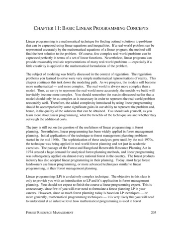
Example 1 LP FormulationMax5x1 7x2s.t.x1 62x1 3x2 19x1 x2 8x1, x2 0Example 1 Graphical Solutionx2x1 x2 88Max 5x1 7x27x1 665Optimal:x1 5, x2 3, z 46432x1 3x2 192112345678910x13

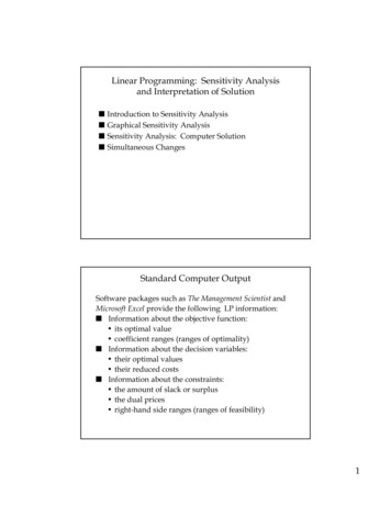
Objective Function Coefficients Let us consider how changes in the objective functioncoefficients might affect the optimal solution. The range of optimality for each coefficient provides therange of values over which the current solution willremain optimal. Managers should focus on those objective coefficientsthat have a narrow range of optimality and coefficientsnear the endpoints of the range.Example 1 Changing Slope of Objective 4

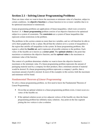
Range of Optimality Graphically, the limits of a range of optimality arefound by changing the slope of the objective functionline within the limits of the slopes of the bindingconstraint lines. The slope of an objective function line, Max c1x1 c2x2,is -c1/c2, and the slope of a constraint, a1x1 a2x2 b, is-a1/a2.Example 1 Range of Optimality for c1The slope of the objective function line is -c1/c2.The slope of the first binding constraint, x1 x2 8, is -1and the slope of the second binding constraint, x1 3x2 19, is -2/3.Find the range of values for c1 (with c2 staying 7)such that the objective function line slope lies betweenthat of the two binding constraints:-1 -c1/7 -2/3Multiplying through by -7 (and reversing theinequalities):14/3 c1 75

Example 1 Range of Optimality for c2Find the range of values for c2 ( with c1 staying 5)such that the objective function line slope lies betweenthat of the two binding constraints:-1 -5/c2 -2/3Multiplying by -1:Inverting,1 5/c2 2/31 c2/5 3/2Multiplying by 5:5 c2 15/2Example 1 Range of Optimality for c1 and c26

Right-Hand Sides Let us consider how a change in the right-hand side fora constraint might affect the feasible region and perhapscause a change in the optimal solution. The improvement in the value of the optimal solutionper unit increase in the right-hand side is called thedual price. The range of feasibility is the range over which the dualprice is applicable. As the RHS increases, other constraints will becomebinding and limit the change in the value of theobjective function.Dual Price Graphically, a dual price is determined by adding 1 tothe right hand side value in question and then resolvingfor the optimal solution in terms of the same twobinding constraints. The dual price is equal to the difference in the values ofthe objective functions between the new and originalproblems. The dual price for a nonbinding constraint is 0. A negative dual price indicates that the objectivefunction will not improve if the RHS is increased.7

Relevant Cost and Sunk Cost A resource cost is a relevant cost if the amount paid forit is dependent upon the amount of the resource usedby the decision variables. Relevant costs are reflected in the objective functioncoefficients. A resource cost is a sunk cost if it must be paidregardless of the amount of the resource actually usedby the decision variables. Sunk resource costs are not reflected in the objectivefunction coefficients.A Cautionary Noteon the Interpretation of Dual Prices Resource cost is sunkThe dual price is the maximum amount you should bewilling to pay for one additional unit of the resource. Resource cost is relevantThe dual price is the maximum premium over thenormal cost that you should be willing to pay for oneunit of the resource.8

Example 1 Dual PricesConstraint 1: Since x1 6 is not a binding constraint,its dual price is 0.Constraint 2: Change the RHS value of the secondconstraint to 20 and resolve for the optimal pointdetermined by the last two constraints:2x1 3x2 20 and x1 x2 8.The solution is x1 4, x2 4, z 48. Hence, thedual price znew - zold 48 - 46 2.Example 1 Dual PricesConstraint 3: Change the RHS value of the thirdconstraint to 9 and resolve for the optimal pointdetermined by the last two constraints: 2x1 3x2 19and x1 x2 9.The solution is: x1 8, x2 1, z 47.The dual price is znew - zold 47 - 46 1.9

Example 1 Dual PricesAdjustable CellsCell B 8 C 8Final ReducedName traintsFinalShadowCell Name ValuePrice B 13 #150 B 14 #2192 B 15 #381Constraint AllowableR.H. SideIncrease61E 301958 0.33333333AllowableDecrease111.66666667Range of Feasibility The range of feasibility for a change in the right handside value is the range of values for this coefficient inwhich the original dual price remains constant. Graphically, the range of feasibility is determined byfinding the values of a right hand side coefficient suchthat the same two lines that determined the originaloptimal solution continue to determine the optimalsolution for the problem.10

Example 1 Range of FeasibilityAdjustable CellsCell B 8 C 8Final ReducedName traintsFinalShadowCell Name ValuePrice B 13 #150 B 14 #2192 B 15 #381Constraint AllowableR.H. SideIncrease61E 301958 0.33333333AllowableDecrease111.66666667Example 2: Olympic Bike Co.Olympic Bike is introducing two new lightweightbicycle frames, the Deluxe and the Professional, to bemade from special aluminum and steel alloys. Theanticipated unit profits are 10 for the Deluxe and 15 forthe Professional. The number of pounds of each alloyneeded per frame is summarized below. A supplierdelivers 100 pounds of the aluminum alloy and 80pounds of the steel alloy weekly.DeluxeProfessionalAluminum Alloy24Steel Alloy32How many Deluxe and Professional frames shouldOlympic produce each week?11

Example 2: Olympic Bike Co. Model Formulation Verbal Statement of the Objective FunctionMaximize total weekly profit. Verbal Statement of the ConstraintsTotal weekly usage of aluminum alloy 100 pounds.Total weekly usage of steel alloy 80 pounds. Definition of the Decision Variablesx1 number of Deluxe frames produced weekly.x2 number of Professional frames produced weekly.Example 2: Olympic Bike Co. Model Formulation (continued)Max 10x1 15x2(Total Weekly Profit)s.t.(Aluminum Available)(Steel Available)2x1 4x2 1003x1 2x2 80x1, x2 012

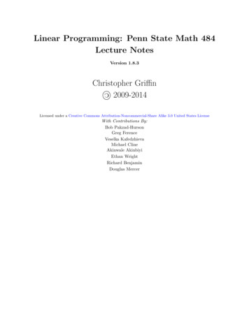
Example 2: Olympic Bike Co. Partial Spreadsheet Showing Problem DataExample 2: Olympic Bike Co. Partial Spreadsheet Showing Solution13

Example 2: Olympic Bike Co. Optimal SolutionAccording to the output:x1 (Deluxe frames) 15x2 (Professional frames) 17.5Objective function value 412.50Example 2: Olympic Bike Co. Range of OptimalityQuestionSuppose the profit on deluxe frames is increased to 20. Is the above solution still optimal? What is thevalue of the objective function when this unit profit isincreased to 20?14

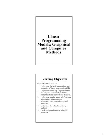
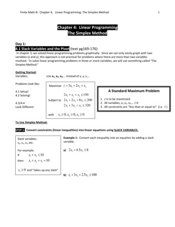
Example 2: Olympic Bike Co. Sensitivity ReportExample 2: Olympic Bike Co. Range of OptimalityAnswerThe output states that the solution remains optimalas long as the objective function coefficient of x1 isbetween 7.5 and 22.5. Since 20 is within this range, theoptimal solution will not change. The optimal profitwill change: 20x1 15x2 20(15) 15(17.5) 562.50.15

Example 2: Olympic Bike Co. Range of OptimalityQuestionIf the unit profit on deluxe frames were 6 insteadof 10, would the optimal solution change?Example 2: Olympic Bike Co. Range of Optimality16

Example 2: Olympic Bike Co. Range of OptimalityAnswerThe output states that the solution remains optimalas long as the objective function coefficient of x1 isbetween 7.5 and 22.5. Since 6 is outside this range, theoptimal solution would change.Example 2: Olympic Bike Co. Range of Feasibility and Sunk CostsQuestionGiven that aluminum is a sunk cost, what is themaximum amount the company should pay for 50 extrapounds of aluminum?17

Example 2: Olympic Bike Co. Range of Feasibility and Sunk CostsExample 2: Olympic Bike Co. Range of Feasibility and Sunk CostsAnswerSince the cost for aluminum is a sunk cost, theshadow price provides the value of extra aluminum.The shadow price for aluminum is the same as its dualprice (for a maximization problem). The shadow pricefor aluminum is 3.125 per pound and the maximumallowable increase is 60 pounds. Since 50 is in thisrange, then the 3.125 is valid. Thus, the value of 50additional pounds is 50( 3.125) 156.25.18

Example 2: Olympic Bike Co. Range of Feasibility and Relevant CostsQuestionIf aluminum were a relevant cost, what is themaximum amount the company should pay for 50 extrapounds of aluminum?AnswerIf aluminum were a relevant cost, the shadow pricewould be the amount above the normal price ofaluminum the company would be willing to pay. Thusif initially aluminum cost 4 per pound, then additionalunits in the range of feasibility would be worth 4 3.125 7.125 per pound.Example 3 Consider the following linear program:Mins.t.6x1 9x2( cost)x1 2x2 810x1 7.5x2 30x2 2x1, x2 019

Example 3 The Management Scientist OutputOBJECTIVE FUNCTION VALUE 27.000Variablex1x2Value1.5002.000Reduced 0.000Dual Price0.000-0.600-4.500Example 3 The Management Scientist Output (continued)OBJECTIVE COEFFICIENT RANGESVariable Lower Limit Current Valuex10.0006.000x24.5009.000Upper Limit12.000No LimitRIGHTHAND SIDE RANGESConstraint Lower Limit Current Value15.5008.000215.00030.00030.0002.000Upper LimitNo Limit55.0004.00020

Example 3 Optimal SolutionAccording to the output:x1 1.5x2 2.0Objective function value 27.00Example 3 Range of OptimalityQuestionSuppose the unit cost of x1 is decreased to 4. Is thecurrent solution still optimal? What is the value of theobjective function when this unit cost is decreased to 4?21

Example 3 The Management Scientist OutputOBJECTIVE COEFFICIENT RANGESVariable Lower Limit Current Valuex10.0006.0004.5009.000x2Upper Limit12.000No LimitRIGHTHAND SIDE RANGESConstraint Lower Limit Current Value15.5008.000215.00030.00030.0002.000Upper LimitNo Limit55.0004.000Example 3 Range of OptimalityAnswerThe output states that the solution remains optimalas long as the objective function coefficient of x1 isbetween 0 and 12. Since 4 is within this range, theoptimal solution will not change. However, the optimaltotal cost will be affected: 6x1 9x2 4(1.5) 9(2.0) 24.00.22

Example 3 Range of OptimalityQuestionHow much can the unit cost of x2 be decreasedwithout concern for the optimal solution changing?Example 3 The Management Scientist OutputOBJECTIVE COEFFICIENT RANGESVariable Lower Limit Current Valuex10.0006.000x24.5009.000Upper Limit12.000No LimitRIGHTHAND SIDE RANGESConstraint Lower Limit Current Value15.5008.000215.00030.00030.0002.000Upper LimitNo Limit55.0004.00023

Example 3 Range of OptimalityAnswerThe output states that the solution remains optimalas long as the objective function coefficient of x2 doesnot fall below 4.5.Example 3 Range of FeasibilityQuestionIf the right-hand side of constraint 3 is increased by1, what will be the effect on the optimal solution?24