Transcription
Deep Vectorization of Technical Drawings?Vage Egiazarian1 [0000 0003 4444 9769] , Oleg Voynov1 [0000 0002 3666 9166] ,Alexey Artemov1[0000 0001 5451 7492] , Denis Volkhonskiy1[0000 0002 9463 7883] ,Aleksandr Safin1[0000 0002 5453 1101] , Maria Taktasheva1[0000 0001 6907 5922] ,Denis Zorin2,1 , and Evgeny Burnaev1[0000 0001 8424 0690]12Skolkovo Institute of Science and Technology, 3 Nobel Street, Skolkovo 143026,Russian FederationNew York University, 70 Washington Square South, New York NY 10012, USA{vage.egiazarian, oleg.voinov, a.artemov, denis.volkhonskiy,aleksandr.safin, maria.taktasheva }@skoltech.ru, /3ddl/projects/vectorizationAbstract. We present a new method for vectorization of technical linedrawings, such as floor plans, architectural drawings, and 2D CAD images. Our method includes (1) a deep learning-based cleaning stage toeliminate the background and imperfections in the image and fill in missing parts, (2) a transformer-based network to estimate vector primitives,and (3) optimization procedure to obtain the final primitive configurations. We train the networks on synthetic data, renderings of vector linedrawings, and manually vectorized scans of line drawings. Our methodquantitatively and qualitatively outperforms a number of existing techniques on a collection of representative technical drawings.Keywords: transformer network, vectorization, floor plans, technicaldrawings1IntroductionVector representations are often used for technical images, such as architecturaland construction plans and engineering drawings. Compared to raster images,vector representations have a number of advantages. They are scale-independent,much more compact, and, most importantly, support easy primitive-level editing.These representations also provide a basis for higher-level semantic structurein drawings (e.g., with sets of primitives hierarchically grouped into semanticobjects).However, in many cases, technical drawings are available only in raster form.Examples include older drawings done by hand, or for which only the hard copyis available, and the sources were lost, or images in online collections. When the?Equal contribution
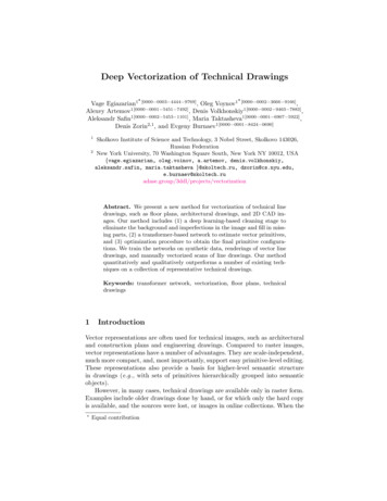
2V. Egiazarian and O. Voynov et al.Fig. 1: An overview of our vectorization method. First, the input image is cleanedwith a deep CNN. Then, the clean result is split into patches, and primitiveplacement in each patch is estimated with with a deep neural network. Afterthat, the primitives in each patch are refined via iterative optimization. Finally,the patches are merged together into a single vector image.vector representation of a drawing document is unavailable, it is reconstructed,typically by hand, from scans or photos. Conversion of a raster image to a vectorrepresentation is usually referred to as vectorization.While different applications have distinct requirements for vectorized drawings, common goals for vectorization are:– approximate the semantically or perceptually important parts of the inputimage well;– remove, to the extent possible, the artifacts or extraneous data in the images,such as missing parts of line segments and noise;– minimize the number of used primitives, producing a compact and easilyeditable representation.We note that the first and last requirements are often conflicting. E.g., inthe extreme case, for a clean line drawing, 100% fidelity can be achieved by“vectorizing” every pixel with a separate line.In this paper, we aim for geometrically precise and compact reconstructionof vector representations of technical drawings in a fully automatic way. Distinctive features of the types of drawings we target include the prevalence ofsimple shapes (line segments, circular arcs, etc.) and relative lack of irregularities (such as interruptions and multiple strokes approximating a single line)other than imaging flaws. We develop a system which takes as input a technicaldrawing and vectorizes it into a collection of line and curve segments (Figure 1).Its elements address vectorization goals listed above. The central element is adeep-learning accelerated optimization method that matches geometric primitives to the raster image. This component addresses the key goal of finding acompact representation of a part of the raster image (a patch) with few vectorprimitives. It is preceded by a learning-based image preprocessing stage, thatremoves background and noise and performs infill of missing parts of the image,and is followed by a simple heuristic postprocessing stage, that further reducesthe number of primitives by merging the primitives in adjacent patches.
Deep Vectorization of Technical Drawings3Our paper includes the following contributions:1. We develop a novel vectorization method. It is based on a learnable deepvectorization model and a new primitive optimization approach. We usethe model to obtain an initial vector approximation of the image, and theoptimization produces the final result.2. Based on the proposed vectorization method, we demonstrate a completevectorization system, including a preprocessing learning-based cleaning stepand a postprocessing step aiming to minimize the number of primitives.3. We conduct an ablation study of our approach and compare it to severalstate-of-the-art methods.2Related workVectorization. There is a large number of methods for image and line drawingvectorization. However, these methods solve somewhat different, often imprecisely defined versions of the problem and target different types of inputs andoutputs. Some methods assume clean inputs and aim to faithfully reproduce allgeometry in the input, while others aim, e.g., to eliminate multiple close linesin sketches. Our method is focused on producing an accurate representation ofinput images with mathematical primitives.One of the widely used methods for image vectorization is Potrace [33]. Itrequires a clean, black-and-white input and extracts boundary curves of darkregions, solving a problem different from ours (e.g., a single line or curve segmentis always represented by polygon typically with many sides). Recent works [27,21]use Potrace as a stage in their algorithms.Another widely used approach is based on curve network extraction andtopology cleanup [11,3,28,6,5,29,17]. The method of [11] creates the curve network with a region-based skeleton initialization followed by morphological thinning. It allows to manually tune the simplicity of the result trading off its fidelity.The method of [3] uses a polyvector field (crossfield) to guide the orientation ofprimitives. It applies a sophisticated set of tuneable heuristics which are difficultto tune to produce clean vectorizations of technical drawings with a low number of primitives. The authors of [28] focus on speeding up sketch vectorizationwithout loss of accuracy by applying an auxiliary grid and a summed area table.We compare to [3] and [11] which we found to be the best-performing methodsin this class.Neural network-based vectorization. To get the optimal result, the methodslike [3,11] require manual tuning of hyper-parameters for each individual inputimage. In contrast, the neural network-based approach that we opt for is designedto process large datasets without tuning.The method of [24] generates vectorized, semantically annotated floor plansfrom raster images using neural networks. At vectorization level, it detects alimited set of axis-aligned junctions and merges them, which is specific to asubset of floor plans (e.g., does not handle diagonal or curved walls).
4V. Egiazarian and O. Voynov et al.In [10] machine learning is used to extract a higher-level representation froma raster line drawing, specifically a program generating this drawing. This approach does not aim to capture the geometry of primitives faithfully and isrestricted to a class of relatively simple diagrams.A recent work [13] focuses on improving the accuracy of topology reconstruction. It extracts line junctions and the centerline image with a two headedconvolutional neural network, and then reconstructs the topology at junctionswith another neural network.The algorithm of [12] has similarities to our method: it uses a neural networkbased initialization for a more precise geometry fit for Bézier curve segments.Only simple input data (MNIST characters) are considered for line drawingreconstruction. The method was also applied to reconstructing 3D surfaces ofrevolution from images.An interesting recent direction is generation of sketches using neural networksthat learn a latent model representation for sketch images [14,39,18]. In principle,this approach can be used to approximate input raster images, but the geometricfidelity, in this case, is not adequate for most applications. In [38] an algorithm forgenerating collections of color strokes approximating an input photo is described.While this task is related to line drawing vectorization it is more forgiving interms of geometric accuracy and representation compactness.We note that many works on vectorization focus on sketches. Although theline between different types of line drawings is blurry, we found that methodsfocusing exclusively on sketches often produce less desirable results for technicalline drawings (e.g., [11] and [9]).Vectorization datasets. Building a large-scale real-world vectorization datasetis costly and time-consuming [23,35]. One may start from raster dataset andcreate a vector ground-truth by tracing the lines manually. In this case, bothlocation and the style may be difficult to match to the original drawing. Anotherway is to start from the vector image and render the raster image from it. Thisapproach does not necessarily produce realistic raster images, as degradation suffered by real-world documents are known to be challenging to model [20]. As aresult, existing vectorization-related datasets either lack vector annotation (e.g.,CVC-FP [16], Rent3D [25], SydneyHouse [7], and Raster-to-Vector [24] all provide semantic segmentation masks for raster images but not the vector groundtruth) or are synthetic (e.g., SESYD [8], ROBIN [34], and FPLAN-POLY [31]).Image preprocessing. Building a complete vectorization system based on ourapproach requires the initial preprocessing step that removes imaging artefacts.Preprocessing tools available in commonly used graphics editors require manualparameter tuning for each individual image. For a similar task of conversion ofhand-drawn sketches into clean raster line drawings the authors of [35,32] useconvolutional neural networks trained on synthetic data. The authors of [23]use a neural network to extract structural lines (e.g., curves separating imageregions) in manga cartoon images. The general motivation behind the networkbased approach is that a convolutional neural network automatically adapts to
Deep Vectorization of Technical Drawings5different types of images and different parts of the image, without individualparameter tuning. We build our preprocessing step based on the ideas of [23,35].Other related work. Methods solving other vectorization problems include,e.g., [37,19], which approximate an image with adaptively refined constant colorregions with piecewise-linear boundaries; [26] which extracts a vector representation of road networks from aerial photographs; [4] which solves a similar problem and is shown to be applicable to several types of images. These methods usestrong build-in priors on the topology of the curve networks.3Our vectorization systemOur vectorization system, illustrated in Figure 1, takes as the input a rastertechnical drawing cleared of text and produces a collection of graphical primitivesdefined by the control points and width, namely line segments and quadraticBézier curves. The processing pipeline consists of the following steps:1. We preprocess the input image, removing the noise, adjusting its contrast,and filling in missing parts;2. We split the cleaned image into patches and for each patch estimate theinitial primitive parameters;3. We refine the estimated primitives aligning them to the cleaned raster;4. We merge the refined predictions from all patches.3.1Preprocessing of the input raster imageThe goal of the preprocessing step is to convert the raw input data into a rasterimage with clear line structure by eliminating noise, infilling missing parts oflines, and setting all background/non-ink areas to white. This task can be viewedas semantic image segmentation in that the pixels are assigned the backgroundor foreground class. Following the ideas of [23,35], we preprocess the input imagewith U-net [30] architecture, which is widely used in segmentation tasks.We trainour preprocessing network in the image-to-image mode with binary cross-entropyloss.3.2Initial estimation of primitivesTo vectorize a clean raster technical drawing, we split it into patches and for eachpatch independently estimate the primitives with a feed-forward neural network.The division into patches increases efficiency, as the patches are processed inparallel, and robustness of the trained model, as it learns on simple structures.64 64We encode each patch Ip [0, 1]with a ResNet-based [15] feature eximtractor X ResNet (Ip ), and then decode the feature embeddings of theprimitives Xipr using a sequence of ndec Transformer blocks [36] prXipr Transformer Xi 1, X im Rnprim demb ,i 1, . . . , ndec .(1)
6V. Egiazarian and O. Voynov et al.Each row of a feature embedding represents one of the nprim estimated primitives with a set of demb hidden parameters. The use of Transformer architectureallows to vary the number of output primitives per patch. The maximum number of primitives is set with the size of the 0th embedding X0pr Rnprim demb ,initialized with positional encoding, as described in [36]. While the number ofprimitives in a patch is a priori unknown, more than 97% of patches in our datacontain no more than 10 primitives. Therefore, we fix the maximum number ofprimitives and filter out the excess predictions with an additional stage. Specifically, we pass the last feature embedding to a fully-connected block, whichextracts the coordinates of the control points, the widths of the primitivesnprimnΘ {θk (xk,1 , yk,1 , . . . , wk )}k 1, and the confidence values p [0, 1] prim .The latter indicate that the primitive should be discarded if the value is lowerthan 0.5. We detail more on the network in supplementary.Loss function. We train the primitive extraction network with the multi-taskloss function composed of binary cross-entropy of the confidence and a weightedsum of L1 and L2 deviations of the parameters L p, p̂, Θ, Θ̂ 1nprimnprimX Lcls (pk , p̂k ) Lloc θk , θ̂k ,(2)k 1Lcls (pk , p̂k ) p̂k log pk (1 p̂k ) log (1 pk ), Lloc θk , θ̂k (1 λ) kθk θ̂k k1 λkθk θ̂k k22 .(3)(4)The target confidence vector p̂ is all ones, with zeros in the end indicatingplaceholder primitives, all target parameters θ̂k of which are set to zero. Sincethis function is not invariant w.r.t. to permutations of the primitives and theircontrol points, we sort the endpoints in each target primitive and the targetprimitives by their parameters lexicographically.3.3Refinement of the estimated primitivesWe train our primitive extraction network to minimize the average deviation ofthe primitives on a large dataset. However, even with small average deviation,individual estimations may be inaccurate. The purpose of the refinement step isto correct slight inaccuracies in estimated primitives.To refine the estimated primitives and align them to the raster image, wedesign a functional that depends on the primitive parameters and raster imageand iteratively optimize it w.r.t. the primitive parametersΘref argmin E (Θ, Ip ) .(5)ΘWe use physical intuition of attracting charges spread over the area of the primitives and placed in the filled pixels of the raster image. To prevent alignment ofdifferent primitives to the same region, we model repulsion of the primitives.
Deep Vectorization of Technical Drawings7We define the optimized functional as the sum of three terms per primitivenprimE Θpos,ΘsizeX , Ip Eksize Ekpos Ekrdn ,(6)k 1 nprimnprimare the primitive position parameters, Θsize θksize k 1where Θpos {θkpos }k 1 are the size parameters, and θk θkpos , θksize .We define the position of a line segment by the coordinates of its midpointand inclination angle, and the size by its length and width. For a curve arc, wedefine the midpoint at the intersection of the curve and the bisector of the anglebetween the segments connecting the middle control point and the endpoints.We use the lengths of these segments, and the inclination angles of the segmentsconnecting the “midpoint” with the endpoints.Charge interactions. We base different parts of our functional on the energyof interaction of unit point charges r1 , r2 , defined as a sum of close- and far-rangepotentialsϕ (r1 , r2 ) e kr1 r2 k22Rc λf e kr1 r2 k2R2f,(7)parameters Rc , Rf , λf of which we choose experimentally. The energy of interaction of the uniform positively charged area of the k th primitive Ωk and a grid ofnpixpoint charges q {qi }i 1at the pixel centers ri is then defined by the followingequation, that we integrate analytically for linesnpixEk (q) XZZqii 1ϕ (r, ri ) dr.2(8)ΩkWe approximate it for curves as the sum of integrals over the segments of thepolyline flattening this curve.In our functional we use three different charge grids, encoded as vectorsof length npix : q̂ represents the raster image with charge magnitudes set tointensities of the pixels, qk represents the rendering of the k th primitive with itscurrent values of parameters, and q represents the rendering of all the primitivesin the patch. The charge grids qk and q are updated at each iteration.Energy terms. Below, we denote the componentwise product of vectors with ,and the vector of ones of an appropriate size with 1.The first term is responsible for growing the primitive to cover filled pixelsand shrinking it if unfilled pixels are covered, with fixed position of the primitive:Eksize Ek ([q q̂]ck q k[1 ck ]) .(9)The weighting ck,i {0, 1} enforces coverage of a continuous raster region following the form and orientation of the primitive. We set ck,i to 1 inside thelargest region aligned with the primitive with only shaded pixels of the raster,
8V. Egiazarian and O. Voynov et al.as we detail in supplementary. For example, for a line segment, this region is arectangle centered at the midpoint of the segment and aligned with it.The second term is responsible for alignment of fixed size primitivesEkpos Ek ([q qk q̂][1 3ck ]) .(10)The weighting here adjusts this term with respect to the first one, and subtraction of the rendering of the k th primitive from the total rendering of the patchensures that transversal overlaps are not penalized.The last term is responsible for collapse of overlapping collinear primitives;for this term, we use λf 0: rdn2Ekrdn Ek qkrdn , qk,i exp [ lk,i · mk,i 1] β kmk,i k,(11)thwhere lk,iP is the direction of the primitive at its closest point to the i pixel,mk,i j6 k lj,i qj,i is the sum of directions of all the other primitives weighted 2w.r.t. their “presence”, and β (cos 15 1) is chosen experimentally.As our functional is based on many-body interactions, we can use an approximation well-known in physics — mean field theory. This translates intothe observation that one can obtain an approximate solution of (5) by viewinginteractions of each primitive with the rest as interactions with a static set ofcharges, i.e., viewing each energy term Ekpos , Eksize , Ekrdn as depending only onthe parameters of the k th primitive. This enables very efficient gradient computation for our functional, as one needs to differentiate each term w.r.t. a smallnumber of parameters only. We detail on this heuristic in supplementary.We optimize the functional (6) by Adam. For faster convergence, every fewiterations we join lined up primitives by stretching one and collapsing the rest,and move collapsed primitives into uncovered raster pixels.3.4Merging estimations from all patchesTo produce the final vectorization, we merge the refined primitives from thewhole image with a straightforward heuristic algorithm. For lines, we link twoprimitives if they are close and collinear enough but not almost parallel. Afterthat, we replace each connected group of linked primitives with a single leastsquares line fit to their endpoints. Finally, we snap the endpoints of intersectingprimitives by cutting down the “dangling” ends shorter than a few percent of thetotal length of the primitive. For Bézier curves, for each pair of close primitiveswe estimate a replacement curve with least squares and replace the original pairwith the fit if it is close enough. We repeat this operation for the whole imageuntil no more pairs allow a close fit. We detail on this process in supplementary.4Experimental evaluationWe evaluate two versions of our vectorization method: one operating with linesand the other operating with quadratic Bézier curves. We compare our method
Deep Vectorization of Technical Drawings9Fig. 2: (a) Ground-truth vector image, and artefacts w.r.t. which we evaluate thevectorization performance (b) skeleton structure deviation, (c) shape deviation,(d) overparameterization.against FvS [11], CHD [9], and PVF [3]. We evaluate the vectorization performance with four metrics that capture artefacts illustrated in Figure 2.Intersection-over-Union (IoU) reflects deviations in two raster shapes1 R2or rasterized vector drawings R1 and R2 via IoU(R1 , R2 ) RR1 R2 . It doesnot capture deviations in graphical primitives that have similar shapes but areslightly offset from each other.Hausdorff distance dH (X, Y ) max sup inf d(x, y), sup inf d(x, y)x X y Yy Y x X,(12)and Mean Minimal Deviation 1 fdM (X Y ) dfM (Y X) ,2, ZZdfinf d(x, y)dXdXM (X Y ) dM (X, Y ) y Yx X(13a)(13b)x Xmeasure the difference in skeleton structures of two vector images X and Y ,where d(x, y) is Euclidean distance between a pair of points x, y on skeletons.In practice, we densely sample the skeletons and approximate these metrics ona pair of point clouds.Number of Primitives #P measures the complexity of the vector drawing.4.1Clean line drawingsTo evaluate our vectorization system on clean raster images with precisely knownvector ground-truth we collected two datasets.To demonstrate the performance of our method with lines, we compiled PFPvector floor plan dataset of 1554 real-world architectural floor plans from acommercial website [2].To demonstrate the performance of our method with curves, we compiledABC vector mechanical parts dataset using 3D parametric CAD modelsfrom ABC dataset [22]. They have been designed to model mechanical partswith sharp edges and well defined surface. We prepared 10k vector images viaprojection of the boundary representation of CAD models with the open-sourcesoftware Open Cascade [1].
10V. Egiazarian and O. Voynov et al.Fig. 3: Examples of synthetic training data for our primitive extraction network.Fig. 4: Sample from DLD dataset: (a) raw input image, (b) the image cleanedfrom background and noise, (c) final target with infilled lines.We trained our primitive extraction network on random 64 64 crops, withrandom rotation and scaling. We additionally augmented PFP with syntheticdata, illustrated in Figure 3.For evaluation, we used 40 hold-out images from PFP and 50 images fromABC with resolution 2000 3000 and different complexity per pixel. We specifyimage size alongside each qualitative result. We show the quantitative results ofthis evaluation in Table 1 and the qualitative results in Figures 5 and 6. Sincethe methods we compare with produce widthless skeleton, for fair comparisonw.r.t. IoU we set the width of the primitives in their outputs equal to the averageon the image.There is always a trade-off between the number of primitives in the vectorizedimage and its precision, so the comparison of the results with different numberprimitives is not to fair. On PFP, our system outperforms other methods w.r.t. allmetrics, and only loses in primitive count to FvS. On ABC, PVF outperforms ourfull vectorization system w.r.t. IoU, but not our vectorization method withoutmerging, as we discuss below in ablation study. It also produces much moreprimitives than our method.4.2Degraded line drawingsTo evaluate our vectorization system on real raster technical drawings, we compiled Degraded line drawings dataset (DLD) out of 81 photos and scansof floor plans with resolution 1300 1000. To prepare the raster targets, wemanually cleaned each image, removing text, background, and noise, and refinedthe line structure, inpainting gaps and sharpening edges (Figure 4).
Deep Vectorization of Technical DrawingsPFPIoU,% dH , px dM , pxFvS [11]313812.8CHD [9]222142.1PVF [3]602041.5Our86/88250.211ABCDLD#P IoU,% dH , px dM , px #P IoU,% #P69665381.763121460911094732938k89170.7 78181331 77/77190.697 79/82 452Table 1: Quantitative results of vectorization. For our method we report twovalues of IoU: with the average primitive width and with the predicted.1770 px256 pxFvS [11]29% / 415px4.2px / 615CHD [9]21% / 215px1.9px / 1192PVF [3]64% / 140px0.9px / 35kOur method89% / 28px0.2px / 1286Ground truth,#P 1634Fig. 5: Qualitative comparison on a PFP image, and values of IoU / dH / dM /#P with best in bold. Endpoints of the primitives are shown in orange.2686 px386 pxFvS [11]67%/ 32px1.1px/ 79CHD [9]67%/ 7px1.0px/ 108PVF [3]95%/ 4px0.2px/ 9.5kOur method86%/ 5px0.4px/ 139Ground truth,#P 139Fig. 6: Qualitative comparison on an ABC image, and values of IoU / dH / dM/ #P with best in bold. Endpoints of the primitives are shown in orange.
12V. Egiazarian and O. Voynov et al.110 px850 px83 pxInput imageCHD [9], 52% / 349Our method, 78% / 368Fig. 7: Qualitative comparison on a real noisy image, and values of IoU / #Pwith best in bold. Primitives are shown in blue with endpoints in orange on topof the cleaned raster image.MS [35]OurIoU,% PSNR4915.79225.5Table 2: Quantitative evaluation of the preprocessing step.To train our preprocessing network, we prepared the dataset consisting of20000 synthetic pairs of images of resolution 512 512. We rendered the groundtruth in each pair from a random set of graphical primitives, such as lines,curves, circles, hollow triangles, etc. We generated the input image via renderingthe ground truth on top of one of 40 realistic photographed and scanned paperbackgrounds selected from images available online, and degrading the renderingwith random blur, distortion, noise, etc. After that, we fine-tuned the preprocessing network on DLD.For evaluation, we used 15 hold-out images from DLD. We show the quantitative results of this evaluation in Table 1 and the qualitative results in Figure 7.Only CHD allows for degraded input so we compare with this method only. Sincethis method produces widthless skeleton, for fair comparison w.r.t. IoU we setthe width of the primitives in its outputs equal to the average on the image,that we estimate as the sum of all nonzero pixels divided by the length of thepredicted primitives.Our vectorization system outperforms CHD on the real floor plans w.r.t. IoUand produces similar number of primitives.Evaluation of preprocessing network. We separately evaluate our preprocessing network comparing with public pre-trained implementation of MS [35].We show the quantitative results of this evaluation in Table 2 and qualitativeresults in Figure 8. Our preprocessing network keeps straight and repeated linescommonly found in technical drawing while MS produces wavy strokes and tendsto join repeated straight lines, thus harming the structure of the drawing.
Deep Vectorization of Technical Drawings13Fig. 8: Example of preprocessing results: (a) raw input image, (b) output ofMS [35], (c) output of our preprocessing network. Note the tendency of MS tocombine close parallel lines.NNNN RefinementNN Refinement PostprocessingIoU,% dH , px dM , px65521.491190.377190.6#P30924097Table 3: Ablation study on ABC dataset. We compare the results of our methodwith and without refinement and postprocessing4.3Ablation studyTo assess the impact of individual components of our vectorization system onthe results, we obtained the results on the ABC dataset with the full system, thesystem without the postprocessing step, and the system without the postprocessing and refinement steps. We show the quantitative results in Table 3 andthe qualitative results in Figure 9.While the primitive extraction network produces correct estimations on average, some estimations are severely inaccurate, as captured by dH . The refinement step improves all metrics, and the postprocessing step reduces the numberof primitives but deteriorates other metrics due to the trade-off between numberof primitives and accuracy.We note that our vectorization method without the final merging step outperforms other methods on ABC dataset in terms of accuracy metrics.5ConclusionWe presented a four-part system for vectorization of technical line drawings,which produces a collection of graphical primitives defined by the control pointsand width. The first part is the preprocessing neural network that cleans theinput image from artefacts. The second part is the primitive extraction network,trained on a combination of synthetic and real data, which operates on patches
14V. Egiazarian and O. Voynov et al.898 pxNN54%/ 11px0.9px/ 109NN Refinement93%/ 5px0.2px/ 69Full67%/ 5px0.5px/ 25Ground truth,#P 57Fig. 9: Results of our method on an ABC image with and without refinementand postprocessing, and values of IoU / dH / dM / #P with best in bold. Theendpoints of primitives are shown in orange.of the image. It estimates the primitives approximately in the right locationmost of the time, how
While di erent applications have distinct requirements for vectorized draw-ings, common goals for vectorization are: { approximate the semantically or perceptually important parts of the input image well; { remove, to the extent possible, the artifacts or extraneous data in the images, such as missing parts of line segments and noise;