Transcription
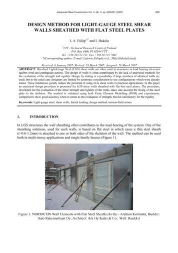
Advanced Steel Construction Vol. 3, No. 3, pp. 628-651 (2007)628DESIGN METHOD FOR LIGHT-GAUGE STEEL SHEARWALLS SHEATHED WITH FLAT STEEL PLATESL.A. Fülöp1,* and I. Hakola1VTT - Technical Research Centre of FinlandP.O. Box 1000, FI-02044 VTTTel. 358 20 722 111; Fax 358 20 722 7001*(Corresponding author: E-mail: Ludovic.Fulop@vtt.fi ; Ilkka.Hakola@vtt.fi)Received: 8 January 2007; Revised: 19 March 2007; Accepted: 28 March 2007ABSTRACT: Sheathed Light-Gauge Steel (LGS) shear walls are often used in structures as load bearing elementsagainst wind and earthquake actions. The design of walls is often complicated by the lack of analytical methods forthe evaluation of the strength and rigidity. Design by testing is a possibility if large numbers of identical walls areused; but in the usual case designers are limited by economic consideration to use configurations which were alreadytested. These limitations greatly reduce the potential of using LGS shear walls in practical applications. In this paperan analytical design procedure is presented for LGS shear walls sheathed with flat thin steel plates. The procedure,developed for the evaluation of the shear strength and rigidity of the walls, takes into account the fixing of the steelplate to the skeleton. The method is validated using both Finite Element Modelling (FEM) and experiments;comparisons show good accuracy when it comes to the evaluation of strength, but not satisfactory for the rigidity.Keywords: Light-gauge steel, shear walls, lateral loading, design method, tension-field action1.INTRODUCTIONIn LGS structures the wall sheathing often contributes to the load bearing of the system. One of thesheathing solutions, used for such walls, is based on flat steel in which cases a thin steel sheath(t 0.6-1.2mm) is attached to one or both sides of the skeleton of the wall. The method can be usedboth in multi-storey applications and single family houses (Figure 1).Figure 1. NORDICON Wall Elements with Flat Steel Sheath (As Oy - Arabian Kotiranta; Builder:Sato Rakennuttajat Oy; Architect: Ark Oy Kahri & Co.; Wall: Ruukki)
629L.A. Fülöp and I. HakolaOne of the particularly interesting applications, in housing, is the use of thin steel cassette sections,Davies [1]. Even if the cassette walls are slightly different from the classical sheathed solutions, theload bearing mechanism is similar. In the case of cassette walls, the connected flanges of thecassettes form the “stud”, while the large webs act as the sheathing (Figure 2).a)b)Figure 2. (a) Steel Skeleton Walls with Flat Steel Sheathing and (b) Cassette Section WallsObviously, the sheathing provides a certain amount of stiffening for the wall, especially if the wallis loaded in shear. Such loading typically occurs in the wall when the structure is subjected to windor earthquake action. In order to design a structure for these actions, the evaluation of the lateralload bearing capacity is required, with a significant part of the strength supplied by the sheathing.The main limitation in the design process comes from the lack of suitable analytical procedures forthe calculation of the capacity and rigidity of the sheathed walls. Design assisted by testing is onepossibility, but it is usually expensive and impractical, due to the diversity of configurations anddimensions of walls in everyday design.In this paper an analytical design procedure is presented for the evaluation of the strength andrigidity of shear walls sheathed with flat steel plates. The procedure takes into account the strengthand the rigidity of the connections between the plate and the frame of the wall, and proved to besufficiently accurate for the evaluation of the strength of the walls, but less reliable for theevaluation of the stiffness. Several particularities of the behaviour of LGS shear walls, usefulduring the design process, are highlighted and critically discussed.2.HISTORICAL DEVELOPMENT OF THE STEEL SHEAR WALLSTo some extent, the calculation methods for classical steel shear walls, used in heavy framestructures, can also be adopted for LGS walls. However, important differences also exist betweenthe two typologies. These differences, and their consequences on the behaviour of the walls, arediscussed in this section.Flat steel plates with larger thickness (t 5-10mm) are sometimes provided in bays of multi-storeysteel frame structures in order to improve the earthquake performance. These shear plates increasethe lateral rigidity and load bearing capacity of the structure, and also contribute to the energydissipation during earthquake. [2].Initially, in these classical applications, the intention was to avoid the elastic buckling of the plates.Until the 1980s, the design limit-state of steel plate shear walls, in North-America, was theout-of-plane buckling of the plate, resulting in the use of very robust walls [3]. Unquestionably,elastic buckling offers inferior performance as compared to plastic failure of the steel plate,especially in terms of dissipative capacity.
Design Method for Light-gauge Steel Shear Walls Sheathed with Flat Steel Plates630Plastic yielding of the plate was facilitated in practical applications by providing out-of-planestiffeners. Besides the out-of-plane stiffeners, two other solutions were proposed with the aim offacilitating plastic failure instead of elastic buckling. The use of low-yield steel, as base material forthe plates, was introduced in Japan [4]; and pure aluminium shear walls were proposed byDeMatteis [5]. In both cases the goal is to exploit the low yield capacity of the material in order tofacilitate shear yielding.Stiffened shear walls were used in most of the early applications in Japan and the USA [6], but thismethod became less popular as it requires large amount of labour for the welding of the stiffeners.An increasing number of recent applications, both in the USA and Canada, use non-stiffened steelplates [6]. In case of non-stiffened walls, elastic buckling is allowed to take place, and the loadresisting mechanism is based on the development of tensile stresses in the already buckled plate,mechanism often referred as tension-field action.The first tension-field theory concerning the post-buckling strength of shear panels was developedby Wagner [7]. Later theories incorporated the bending effect of the marginal beams and shearstresses in the plate [8]. A plastic design method for the classical steel shear walls was presented,for single-storey and multi-story frames, by Berman & Bruneau [3].More recently, Elgaaly [2] proposed an analytical model for the calculation of the capacity of shearwalls with both welded and bolted thin steel plates. The model is based on the concept of replacingthe sheathing with a series of equivalent trusses. For the case of bolted steel plates Elgaaly [2]suggested, that the shear wall should be designed so that the yielding of the plate, and not thecapacity of the end connections, should control the failure of the shear wall. It will be shown laterin this paper, that this condition can hardly, if at all, be fulfilled with LGS shear walls.In the case of LGS walls, it is also not possible to avoid the elastic buckling, due to the extremethinness of the plate. If we would include LGS shear plates in the slenderness chart presented byAstaneh-Asl [6], they would form a group of “extremely slender” plates with very largewidth-to-thickness ratios (L/t 600-1200, Figure 3). Therefore, the use of stiffeners or low-yieldmaterial is not feasible, and the storey shear has to be transmitted by the tension-field action only.VτyτyV /V yτyVτyσcr σy1σyσcrVσyσyCompactNon-compactSlender1.1 k v Efy[60.80]1.37 k v Efy[75.100]ExtremelyExtremly slenderslender[600.1200]h/tFigure 3. Behaviour of Steel Shear Walls (Adapted from Astaneh-Asl [6])
631L.A. Fülöp and I. HakolaThe other difference between classical and LGS walls, is that in the heavy steel applications theplates are usually continuously connected to the frame, most often by welding. But welding israrely used in LGS structures, because of the damage it causes to the zinc coating of the elements,and the connection of the plate is usually in points, by screws or pins.3.CALCULATIONMETHODFORWALLSCONTINUOUSLY CONNECTED TO THE FRAME3.1Basic AssumptionsWITHSTEELPLATESThe calculation of shear walls, covered by thin steel sheathing, is based on the assumption that theshear is resisted by the tension-field action in the plate (Figure 3). Other assumptions include:(i) The skeleton of the wall is pinned. This implies that the connections between studs and tracksdo not transmit bending, and the frame effect of the wall skeleton is negligible.(ii) The bending rigidity of studs and tracks is large, as compared to the rigidity of the thin plate.Therefore, the studs and tracks do not bend significantly during the deformation of the wall.This assumption may be doubtful when it comes to relatively long studs.In the first step of the analysis, the wall panel is divided along the length into cells, which aresheathed with a single steel plate (Figure 4). If the cells are identical, they act in parallel and theshear loading of the wall is transmitted equally to each cell. Since the capacity and rigidity of thecells can be summed, the calculation method for these values has been developed for one cell.7000x 221251251250x 20x 27007002700STEEL SHEETS t 0.6mmGRADE S320GD Z100 overlap24001200Figure 4. Division of Wall Panels into “Cells”Buckling of the plate occurs in the very early stage, and at small forces, due to the very largewidth-to-thickness ratios (L/t 600-1200). However, the buckling force does not represent theultimate capacity of the wall, because the post-buckling path is stable, and the load cansubstantially increase due to tension-field action. An oblique tension stress pattern develops in theplate resembling a pattern of oblique strips subjected to tension (Figure 5.a). These strips yieldgradually, leading to the loss of load bearing capacity of the cell, and of the entire wall.
Design Method for Light-gauge Steel Shear Walls Sheathed with Flat Steel Plates632For analytical purposes, the cells can be divided into finite strips running obliquely and forming anangle α with the vertical. The position of the current strip is defined by its distance from the cornerof the cell (x), while its width is dx (Figure 5.a). The load bearing capacity of the cell is calculatedby supposing that the only mechanism to resist the loading is the strips subjected to stretching.As presented in Figure 5.a, the strips can have different characteristics (e.g. length, axial stiffness),depending on their position in the plate. Based on the geometry, several zones of strips can bedefined. As shown later, the behaviour of strips in the same zone can be described by identicalformulae. In the elastic stage, the structural scheme of this multi-strip model isstaticallyindeterminate, but when all strips yielded classical plastic analysis apply. In the yieldingstage the forces in every strip are known, and equal to the yield resistance of the strip.Finite Element (FE) analyses and experimental evidence suggest that independent yield patternsdevelop for each cell of a wall, thus substantiating the assumption that the cells in a wall actindependently.xdxxVi2BL cos αVi2CdFSZone 1Zone 1αofhhtensilest ressZone 2DirectionαZone 3RHA(a)L(b)ARVADLRHDRVDFigure 5. (a) Differential strips (dx) and Zones, (b) forces in strips from horizontal loads (Vi)3.2Evaluation of the Load Bearing CapacityThe relationship between the tensile force in the strip (dFs) and the horizontal force (Vi) that causesit (Figure 5.b), can be written for strips in Zone 1 as:Vi dFS xh(1)If dFS is interpreted as the resistance of the strip, then Vi will represent the contribution of the stripto the capacity of the cell. The total load bearing capacity contribution of strips in Zone 1 (ViZone1)can be calculated by summing up the contributions of individual strips in the entire Zone 1:
633ViL.A. Fülöp and I. HakolaZone1L cos α x 0dFS xh(2)Similarly the load bearing contributions of all strips in Zone 2 (ViZone2) and Zone 3 (ViZone3) are:ViZone 2 h sin αx L cos αdFS L cos αh(3)ViZone 3 h sin α L cos αx h sin αdFS [(h sin α L cos α ) x ]h(4)By simplifying Eq. (4) it can be shown that the contributions of strips in Zone 1 and Zone 3 areequal. Intuitively it can also be seen that the two zones are identical from the point of view of theload bearing. Therefore:ViZone 3 L cos αx 0dFS xZone1 Vih(5)The total horizontal load bearing capacity of the cell (V), in the stage when all strips yield, is thesum of the contributions of the three zones:V ViZone1 ViZone 2 ViZone 3 2 ViZone1 ViZone 2(6)As the yield resistance of all strips is equal to dFS dA f y t dx f y , the total capacity expressedin Eq.6 can be calculated as:h sin αdFS xdFS L cos α cos αx 0xLhht f y L cosαt f y L cos α h sin α1 2 x dx dx t f y L sin(2α ) x L cos αh x 0h2V 2 L cos α(7)The background of this expression was presented in more detail by Berman and Bruneau [3] forclassical steel shear walls used in multi-storey frames.3.3Evaluation of the RigidityBased on the assumption that the frame is pinned, and made of very rigid bars that do not bend, itcan be noticed that the deformed shape of the cell is geometrically determined (Figure 6). Thismeans that the lengthening and the corresponding force in each strip can be calculated for anyhorizontal displacement of the top. Therefore, the rigidity of the cell can be evaluated.A deformation Δ at the top of the cell causes the points 1 and 2 to displace with Δ1 and Δ2 (Figure 6).If the deformations are small, it can be accepted that the two points have only horizontaldisplacements.
Design Method for Light-gauge Steel Shear Walls Sheathed with Flat Steel Plates63422l12h1α1hl12xα1LFigure 6. Strip in the Deformed Stage of the Cell (Zone 1)The length (l12,Z1) of a strip in Zone 1, at a distance x from the corner, is:l12,Z 1 xsin α cos α(8)The lengthening of the strip (Δl12,Z1) corresponding to the top displacement of Δ can be expressedas:Δl12,Z 1 Δ xh(9)The deformations Δl12,Z1 and Δ can be expressed as a function of the strip force (dFS) and thecontribution of dFS to the load bearing of the wall (Vi):dFSx V iZ 1k s ,Z 1 h dkt(10)Where ks,Z1 is the axial rigidity of the current strip, and dktZ1 is the strips contribution to the shearrigidity of the cell.Also, by using the formula of Vi (Eq. 1), the rigidity contribution of one strip in Zone 1 to thehorizontal rigidity of the cell (dktZ1) can be written:dktZ 1 x2 k s ,Z 1h2(11)Similarly, the length of a strip in Zone 2 (l12,Z2) is:l12,Z 2 Lsin α(12)
635L.A. Fülöp and I. HakolaThe elongation of a strip in Zone 2 (Δl12,Z2):Δl12, Z 2 Δ L cos αh(13)And the contribution of a strip in Zone 2 (dktZ2) to the rigidity of the wall reads:dktZ 2 L2 cos 2 α k s ,Z 2h2(14)The strips in Zone 3 are similar to the ones in Zone 1, their contribution to the rigidity of the cellbeing identical to the ones in Zone 1.The combined rigidity contribution of the strips in Zone 1 to the rigidity of the wall (KZone1) is thesummation of the rigidity contribution of each strip:KZone1 L cos α0dkZ1t L cos α0x2E t L2 sin α cos3 α k s ,Z 1 h22 h2(15)Where the rigidity of strips in Zone 1 (ks,Z1) is: E A E t dx sin α cos αk s ,Z 1 x l12,Z 1 (16)Similarly for Zone 2:K Zone 2 h sin αL cos αdktZ 2 h sin αL cos αL2 cos 2 α k s ,Z 2 h2E t L sin α cos 2 α (h sin α L cos α )h2(17)If the rigidity contributions of the strips in Zones 1, 2 and 3 are summed up, the total rigidity of thecell (KTOT) is obtained as follows:KTOT 2 K Zone1 K Zone 2 3.41 E t L 2 sin (2 α )h4(18)Characteristics of the Plate YieldingIf we suppose that the strips behave in an elastic-plastic manner, it can be shown that all strips inthe cell yield simultaneously at a lateral displacement of the wall Δy.For strips in Zone 1 (and Zone 3) the yield elongation of any strip (Δl12y,Z1) is (using Eq. 8):Δl12 y , Z 1 ε y l12, Z 1 fyx E sin α cos α(19)
Design Method for Light-gauge Steel Shear Walls Sheathed with Flat Steel Plates636For the strips in Zone 2, Δl12y,Z1 is (from Eq. 12):Δl12 y , Z 2 ε y l12, Z 2 fyL E sin α(20)Both of these elongations correspond to a top displacement that can be calculated by expressing Δfrom Eq. (9) and (13), and by substituting into them Δl12y,Z1 and Δl12y,Z2 from Eq. (19) and (20),respectively: h x Δl12 y ,Z 1 f y h1Δy E sin α cos α h Δl12 y ,Z 2 L cos α (21)Therefore, strips yield at the same top horizontal displacement Δy, given by Eq. (21), regardless oftheir position in the cell. Even the yield displacement of the variable length strips in Zone 1 doesnot depend on the position of the strip in the cell. Interesting to note that Δy is linearly dependent onthe height of the cell (h), but not dependent on L.In conclusion, Eq. (7), (18) and (21) express the load bearing capacity (V), the rigidity (KTOT) andthe yield displacement (Δy) of the wall-cell. The wall-cell, modelled with the strip model, haselastic-plastic behaviour, provided that the strips have elastic-plastic behaviour; and only two of thethree equations are independent, while the third can always be expressed from the other two.3.5Evaluation of the Inclination Angle of the Strips (α)As it can be observed in Eq. (7) and (18), in order to calculate the capacity and rigidity of a cell,one should previously determine the inclination of the strips α (Figure 5). Based on FE modelling,corresponding to usual dimensions of the walls, in this paper a proposal is made for the empiricalevaluation of α.For the sake of simplicity Elgaaly [2] suggested that the angle should be taken as α 45 , regardlessof the dimensions of the wall. However, it can be observed that the use of α 45 in Eq. (7) leads toa maximisation of the expression and to an unsafe over-estimation of the design capacity.On the other hand, as early as in Wagner’s [7] work a formulation was presented for the evaluationof α, based on the minimisation of the strain energy accumulated during the deformation. Theformula takes into account the strain energy due to the tension-field in the plate and due to the axialforce in the frame members. Timler and Kulak [8] amended the formula of Wagner by including thebending effect of the frame members. They argued that the bending for members with plate on bothsides (ex. intermediate studs in LGS walls) can be neglected, but for members with plate acting onone side it should be taken into account. This second case applies for marginal studs and tracks inLGS walls. Both proposals neglect the compression and shear stresses in the plate.If the frame members are considered infinitely rigid, both under axial loading and in bending, thestrain energy due to the tension-field action in the plate remains the only factor to be taken intoaccount. In this case, the strain energy is minimum for α 45 independently of the dimensions ofthe plate.
637L.A. Fülöp and I. HakolaHowever, experimental observations and preliminary FEM analyses, using rigid frame members,have shown that this is not the case. In reality α depends on the dimensions of the plate, probablydue to the presence of the compression and shear stresses.A series of FE models have been prepared for the evaluation of α, and for the verification of thecapacity and the rigidity formulae (Eq. 7 & 18). The models, developed in ABAQUS 6.5, consistedof a perfectly pinned frame modelled as beams (Linear line type B31) with the thin steel platemodelled as shell (Quadratic quadrilateral type S8R).The flatness of the plate was locally disturbed close to the midpoint, by a self-balancing pair ofsmall out-of-plane bending moments, before applying lateral loading at the top. Then the cell wassubjected to steadily increasing lateral load at the top, and the yield pattern was left to developwithout further disturbance. The analysis was performed with displacement control, and the modelincluded both geometrical and material non-linearity.In the first stage, the h/L ratio ranged from 1.42 to 6.17 (Table 1). The behaviour of the platematerial was elastic-plastic with fy 210N/mm2 (E 210000N/mm2) and no limitation on the plasticstrain. The thickness of the plate was t 0.6mm, the plate being continuously connected to the frame.The inclination angles, evaluated using the FE models, are summarized in Table 1.Table 1. Cases of Cells Calculated with FEM and 2 12 22 32 42 5170022002700320037006006006006006003 13 23 33 43 5170022002700320037004 14 24 34 44 517002200270032003700h/LIn a second stage, further FE models were developed in order to improve the prediction for theangle. Cells with length of L 600, 900, 1200, 1600mm; width of h 1400, 1800, 2200, 2600, 3000,3400mm, and plate thicknesses of t 0.4; 0.6; 0.8 and 1.2 have been analysed. The yield stress offy 350N/mm2 has been used for the steel plate.
Design Method for Light-gauge Steel Shear Walls Sheathed with Flat Steel Plates638Based on the first set of data the following empirical formulation was proposed by Fülöp [10] forthe evaluation of α:α DEG 45 0.006 (h L)(22)The results of the second set of FE modelling highlighted that the thickness of the sheathing platealso influences the inclination angle. Consequently, an improved form of the equation is proposed,which includes the effect of the plate thickness:α DEG 45 (0.0035 t 0.00263) (h L)(23)The reliability of Eq. 22 and 23 has been evaluated using ER, the average absolute value calculatedfrom the relative error of the predictions, based on the data from the two stages of the analysis. ERand its standard deviation σER are presented in Table 2. A comparison plot of the angles given by theproposed expression (Eq. 23) and the angles evaluated using the FEM is shown in Figure 7.Table 2. Reliability of the Proposed Formula for α (Eq. 22 and 23)Analysis stage121 2PlateFormulathickness (t)Eq. 22AllEq. 23Allt 0.4mmEq. 23t 0.6mmt 0.8mmt 1.2mmAllEq. 5.032.621.527.392.703.553.27It can be noticed in Table 2 that, the values of the error ER are larger for the thicker plates (ex.t 1.2mm). This highlights the fact that, for larger thicknesses, the effect of compression and shearstresses become important, and the behaviour can be less and less accurately described by thetension strip model.It is also notable that the angles evaluated with the first set of FE models (t 0.6mm, fy 210N/mm2)show good fit with Eq. 23 only for some cases (Figure 7). The difference becomes more significantas the h/L ratio increases, as it can be seen also from the larger errors ER and σER (Table 2). Thismay point to the yield stress having an effect on α. However, in practical applications, the range ofthe yield stress of the plate is quite narrow and the resulting variation of the angle not significant.It is important to note again that Eq. 23 is empirical, based on the evaluation of the angle fromFEM, so its accuracy may be uncertain. However, it was judged that this accuracy is enough for theevaluation of the angle in practical cases, especially because α in the expressions for strength (Eq. 7)and stiffness (Eq. 18) is used in trigonometrical functions that reduce the variability in the vicinityof 45 .
639L.A. Fülöp and I. Hakola45 10%αDEG( )40-10%35t 0.6,t 0.4,t 0.6,t 0.8,t 1.2,302525303540fy 210fy 350fy 350fy 350fy 35045αFEM( )Figure 7. Comparison of the Angle α Values. FEM vs. Eq. (23)3.6Validation of the Strength and Rigidity FormulasThe previously presented FE models were also used for the checking of the accuracy of theanalytical formulas for strength (Eq. 7) and rigidity (Eq. 18). The strength (V) and rigidity (KTOT) ofthe cells have been calculated by using Eq. (7) and (18), for the cases corresponding to the first stepof the FE study, and have been compared to the characteristic curves obtained by FEM (Table 1).For example, the nonlinear FEM characteristic curves for the cells with L 1200mm are comparedin Figure 8 with the equivalent elastic-plastic line, based on the analytical rigidity and capacityfrom Table 1.80V (N)60404 14 24 34 44 5200051015Δ (mm)Figure 8. Analytical vs. FEM Curves for Walls with L 1200mmA bump, corresponding to the buckling of the plate, can be observed at the beginning of eachcharacteristic curve obtained by FEM. It can be noticed that the rigidity is higher at the verybeginning of the curves; but once the plate buckles the rigidity decreases, the response stabilizes,and the rest of the curve is purely due to the tension-field action.
Design Method for Light-gauge Steel Shear Walls Sheathed with Flat Steel Plates640According to the analytical formulation (Eq. 21) all strips in the equivalent strip model should yieldat the same lateral displacement Δy. The tendency to have a distinct yield point can also be observedon the characteristic curves obtained by FEM (Figure 8). The effect is more obvious for lower h/Lratios and tends to be attenuated for very high ones.In some cases the prediction of the rigidity is less accurate. The results suggest that the accuracy ofthe strip model decreases as the h/L ratio increases, but the difference between the FEM result andEq. (18) was not more than 20% for the cases presented in Table 1. Of course, very large h/L ratiosare not feasible, and for practical applications the upper limit of h/L 5 is suggested.The rigidity determined by FEM is always bigger than the one calculated analytically. This is due tothe fact that the analytical calculation ignores secondary load transmission by compression or shearstresses in the plate.Overall, both V and KTOT are well predicted by the analytical formulation, suggesting that the stripmodel is adequate to describe the behaviour of the thin plate.4.CALCULATION METHOD FOR WALLS WITH PLATE CONNECTED TO THEFRAME IN POINTSThe expressions presented in the previous chapters are valid only as long as the yielding capacity ofeach individual strips is equal. This is true if the steel plate is connected to the frame continuously.However, if the plate is connected to the frame in points, several failure modes of the plate candevelop, like: (1) the yielding of the plate, (2) the failure of the connections on the vertical edge, (3)net-section failure of the plate in the vertical connection line, (4) failure of the connections on thehorizontal edge, and (5) net-section failure of the plate in the horizontal connection line. Each ofthese failure modes, and the behaviour of the components causing them, has to be taken intoaccount in terms of both capacity and rigidity.4.1Evaluation of the Load Bearing CapacityThe effect of the failure modes can be incorporated in the strength calculation, by assigning, at thestrip level, a characteristic resistance to each mode. The smallest of these characteristic resistanceswill point to the governing failure mode of the strip and will determine its tensile capacity, dFS inEq (1). The practical way to take into account the failure modes is to operate with stresses insteadof forces. In case of each strip, an equivalent yield stress (fy,ech) will correspond to each failuremode, and the smallest of these yield stresses will be the basis for the calculation of the stripresistance ( dFS min( f y ,ech,1 , f y ,ech , 2 .) t dx ). Similar procedure was proposed by Elgaaly [2].All five enumerated failure modes influence the capacity in the case of strips from Zone 1 and 3;but in the case of strips in Zone 2, only the first three modes exist.The equivalent yield stresses corresponding to each failure mode are:(i) The yielding of the strip at force dFS f y t dx is the basic case. The yield stress is fy.(ii) The equivalent stress corresponding to the capacity of the vertically placed connectors can beexpressed as:
641f yV,ech ,s L.A. Fülöp and I. Hakola1FBS S t sin α(24)Where, the capacity of one connector is FBS and the spacing of the connectors is S (Figure 9).ααdxSdxsin αscrew(FbS )(a)(b)FbSSFigure 9. (a) One Screw in the Vertical Row and (b) Characteristics of the Screw Reduced to dxIf the connectors are self-tapping screws, the bearing capacity of a screw is FBS α EC 3 f u d t ,according to prEN-1993-1-3 [11], and Eq. 24 becomes:f yV,ech ,s α EC 3 f u dS sin α(25)It should be noted that only bearing failure of the screws is acceptable, because this failure modeensures ductile behaviour of the wall. Bearing failure is easily obtained as the thickness of the plateis considerably smaller than that of the profiles of the skeleton. Therefore, the joint is a typicalthin-to-thick sheath connection that usually fails by bearing, if the end distances are adequate.(iii) The equivalent stress for net-section failure in the vertical connection line, can be calculated,using the definition of net-section area given in prEN-1993-1-1 [12], when both normal andtangential stresses act on the net-section surface: s2 Anet Agross t n d 4 p (26)The net-section area expression can be adapted for the oblique strips having a width of S (Figure 10):Anet t ( S d ) t S cos 2 α 4 sin α(27)Therefore, based on net-section failure, and reduced to dx width, the capacity of the strip (FVnet) is:1 1 d S tV f u AVnet ,dx f u t dx Fnet4 tan 2 α sin α(28)
Design Method for Light-gauge Steel Shear Walls Sheathed with Flat Steel Plate
ABSTRACT: Sheathed Light-Gauge Steel (LGS) shear walls are often used in structures as load bearing elements against wind and earthquake actions. The design of walls is often complicated by the lack of analytical methods for the evaluation of the strength and rigidity. Design by testing is a possibility if large numbers of identical walls are