Transcription
This page intentionally left blank
Modern Quantum Field TheoryA Concise IntroductionQuantum field theory is a key subject in physics, with applications in particle andcondensed matter physics. Treating a variety of topics that are only briefly touched onin other texts, this book provides a thorough introduction to the techniques of fieldtheory.The book covers Feynman diagrams and path integrals, and emphasizes the pathintegral approach, the Wilsonian approach to renormalization, and the physics of nonabelian gauge theory. It provides a thorough treatment of quark confinement and chiralsymmetry breaking, topics not usually covered in other texts at this level. The StandardModel of particle physics is discussed in detail. Connections with condensed matterphysics are explored, and there is a brief, but detailed, treatment of non-perturbativesemi-classical methods (instantons and solitons).Ideal for graduate students in high energy physics and condensed matter physics, thebook contains many problems, providing students with hands-on experience with themethods of quantum field theory.Thomas Banks is Professor of Physics at the Santa Cruz Institute for Particle Physics(SCIPP), University of California, and NHETC, Rutgers University. He is consideredone of the leaders in high energy particle theory and string theory, and was co-discovererof the Matrix Theory approach to non-perturbative string theory.
Modern Quantum Field TheoryA Concise IntroductionTom BanksUniversity of California, Santa Cruzand Rutgers University
CAMBRIDGE UNIVERSITY PRESSCambridge, New York, Melbourne, Madrid, Cape Town, Singapore, São PauloCambridge University PressThe Edinburgh Building, Cambridge CB2 8RU, UKPublished in the United States of America by Cambridge University Press, New Yorkwww.cambridge.orgInformation on this title: www.cambridge.org/9780521850827 T. Banks 2008This publication is in copyright. Subject to statutory exception and to the provision ofrelevant collective licensing agreements, no reproduction of any part may take placewithout the written permission of Cambridge University Press.First published in print format 2008ISBN-13 978-0-511-42899-9eBook (EBL)ISBN-13hardback978-0-521-85082-7Cambridge University Press has no responsibility for the persistence or accuracy of urlsfor external or third-party internet websites referred to in this publication, and does notguarantee that any content on such websites is, or will remain, accurate or appropriate.
Contents1 Introduction1.1 Preface and conventions1.2 Why quantum field theory?page 1132 Quantum theory of free scalar fields2.1 Local fields2.2 Problems for Chapter 2810133 Interacting field theory3.1 Schwinger–Dyson equations and functional integrals3.2 Functional integral solution of the SD equations3.3 Perturbation theory3.4 Connected and 1-P(article) I(rreducible) Green functions3.5 Legendre’s trees3.6 The Källen–Lehmann spectral representation3.7 The scattering matrix and the LSZ formula3.8 Problems for Chapter 31717202426283032364 Particles of spin 1, and gauge invariance4.1 Massive spinning particles4.2 Massless particles with helicity4.3 Field theory for massive spin-1 particles4.4 Problems for Chapter 438383940435 Spin- 12 particles and Fermi statistics5.1 Dirac, Majorana, and Weyl fields: discrete symmetries5.2 The functional formalism for fermion fields5.3 Feynman rules for Dirac fermions5.4 Problems for Chapter 544495658596 Massive quantum electrodynamics6.1 Free the longitudinal gauge bosons!6.2 Heavy-fermion production in electron–positron annihilation6.3 Interaction with heavy fermions: particle paths andexternal fields62646568
tviContents6.46.5The magnetic moment of a weakly coupled charged particleProblems for Chapter 669747Symmetries, Ward identities, and Nambu–Goldstone bosons7.1 Space-time symmetries7.2 Spontaneously broken symmetries7.3 Nambu–Goldstone bosons in the semi-classical expansion7.4 Low-energy effective field theory of Nambu–Goldstone bosons7.5 Problems for Chapter 77678818485898Non-abelian gauge theory8.1 The non-abelian Higgs phenomenon8.2 BRST symmetry8.3 A brief history of the physics of non-abelian gauge theory8.4 The Higgs model, duality, and the phases of gauge theory8.5 Confinement of monopoles in the Higgs phase8.6 The electro-weak sector of the standard model8.7 Symmetries and symmetry breaking in the strong interactions8.8 Anomalies8.9 Quantization of gauge theories in the Higgs phase8.10 Problems for Chapter 8939697991011031131161181301329Renormalization and effective field theory9.1 Divergences in Feynman graphs9.2 Cut-offs9.3 Renormalization and critical phenomena9.4 The renormalization (semi-)group in field theory9.5 Mathematical (Lorentz-invariant, unitary) quantum field theory9.6 Renormalization of φ 4 field theory9.7 Renormalization-group equations in dimensional regularization9.8 Renormalization of QED at one loop9.9 Renormalization-group equations in QED9.10 Why is QED IR-free?9.11 Coupling renormalization in non-abelian gauge theory9.12 Renormalization-group equations for masses and the hierarchyproblem9.13 Renormalization-group equations for the S-matrix9.14 Renormalization and symmetry9.15 The standard model through the lens of renormalization9.16 Problems for Chapter 913713914214514815415616116417317818110 Instantons and solitons10.1 The most probable escape path10.2 Instantons in quantum mechanics188191193201203206206207
tviiContents10.310.410.510.610.710.810.9Instantons and solitons in field theoryInstantons in the two-dimensional Higgs modelMonopole instantons in three-dimensional Higgs modelsYang–Mills instantonsSolitons’t Hooft–Polyakov monopolesProblems for Chapter 1021321622122623223623911 Concluding remarks242Appendix AAppendix BAppendix CAppendix DAppendix EAppendix F245247248251256260ReferencesAuthor indexSubject indexBooksCross sectionsDiracologyFeynman rulesGroup theory and Lie algebrasEverything else262268269
1Introduction1.1 Preface and conventionsThis book is meant as a quick and dirty introduction to the techniques of quantum fieldtheory. It was inspired by a little book (long out of print) by F. Mandl, which my advisorgave me to read in my first year of graduate school in 1969. Mandl’s book enabled thesmart student to master the elements of field theory, as it was known in the early1960s, in about two intense weeks of self-study. The body of field-theory knowledgehas grown way beyond what was known then, and a book with similar intent has to belarger and will take longer to absorb. I hope that what I have written here will fill thatMandl niche: enough coverage to at least touch on most important topics, but shortenough to be mastered in a semester or less. The most important omissions will besupersymmetry (which deserves a book of its own) and finite-temperature field theory.Pedagogically, this book can be used in three ways. Chapters 1–6 can be used as a textfor a one-semester introductory course, the whole book for a one-year course. In eithercase, the instructor will want to turn some of the starred exercises into lecture material.Finally, the book was designed for self-study, and can be assigned as a supplementarytext. My own opinion is that a complete course in modern quantum field theory needs3–4 semesters, and should cover supersymmetric and finite-temperature field theory.This statement of intent has governed the style of the book. I have tried to be terserather than discursive (my natural default) and, most importantly, I have left manyimportant points of the development for the exercises. The student should not imaginethat he/she can master the material in this book without doing at least those exercisesmarked with a *. In addition, at various points in the text I will invite the reader to provesomething, or state results without proof. The diligent reader will take these as extraexercises. This book may appear to the student to require more work than do texts thattry to spoon-feed the reader. I believe strongly that a lot of the material in quantumfield theory can be learned well only by working with your hands. Reading or listeningto someone’s explanation, no matter how simple, will not make you an adept. My hopeis that the hints in the text will be enough to let the student master the exercises andcome out of this experience with a thorough mastery of the basics.The book also has an emphasis on theoretical ideas rather than application to experiment. This is partly due to the fact that there already exist excellent texts that concentrateon experimental applications, partly due to the desire for brevity, and partly to increase
t2Introductionthe shelf life of the volume. The experiments of today are unlikely to be of intense interest even to experimentalists of a decade hence. The structure of quantum field theorywill exist forever.Throughout the book I use natural units, where h̄ c 1. Everything has units ofsome power of mass/energy. High-energy experiments and theory usually concentrateon the energy range between 10 3 and 103 GeV and I will often use these units. Anotherconvenient unit of energy is the natural one defined by gravitation: the Planck mass,MP 1019 GeV, or reduced Planck mass, mP 2 1018 GeV. The GeV is the naturalunit for hadron masses. Around 0.15 GeV is the scale at which strong interactionsbecome strong. Around 250 GeV is the natural scale of electro-weak interactions, and 2 1016 GeV appears to be the scale at which electro-weak and strong interactionsare unified.I will use non-relativistic normalization, p q δ 3 (p q), for single-particle states.Four-vectors will have names which are single Latin letters, while 3-vectors will bewritten in bold face. I will use Greek mid-alphabet letters for tensor indices, and Latinearly-alphabet letters for spinors. Mid-alphabet Latin letters will be 3-vector components. I will stick to the van der Waerden dot convention (Chapter 5) for distinguishingleft- and right-handed Weyl spinors. As for the metric on Minkowski space, I will usethe West Coast, mostly minus, convention of most working particle theorists (and ofmy toilet training), rather than the East Coast (mostly plus) convention of relativistsand string theorists.Finally, a note about prerequisites. The reader must begin this book with a thoroughknowledge of calculus, particularly complex analysis, and a thorough grounding in nonrelativistic quantum mechanics, which of course includes expert-level linear algebra.Thorough knowledge of special relativity is also assumed. Detailed knowledge of themathematical niceties of operator theory is unnecessary. The reader should be familiarwith the Einstein summation convention and the totally anti-symmetric Levi-Civitasymbol a1 .an . We use the convention 0123 1 in Minkowski space. It would be usefulto have a prior knowledge of the theory of Lie groups and algebras, at a physics level ofrigor, although we will treat some of this material in the text and Appendix G. I havesupplied some excellent references [1–4] because this math is crucial to much that wewill do. As usual in physics, what is required of your mathematical background is aknowledge of terminology and how to manipulate and calculate, rather than intimatefamiliarity with rigor and formal proofs.1.1.1 AcknowledgementsI mostly learned field theory by myself, but I want to thank Nick Wheeler of ReedCollege for teaching me about path integrals and the beauties of mathematical physics ingeneral. Roman Jackiw deserves credit for handing me Mandl’s book, and Carl Benderhelped me figure out what an instanton was before the word was invented. Perhaps themost important influence in my grad school years was Steven Weinberg, who taughtme his approach to fields and particles, and everything there was to know about broken
t31.2 Why quantum field theory?symmetry. Most of the credit for teaching me things about field theory goes to LennySusskind, from whom I learned Wilson’s approach to renormalization, lattice gaugetheory, and a host of other things throughout my career. Shimon Yankielowicz andEliezer Rabinovici were my most important collaborators during my years in Israel.We learned a lot of great physics together. During the 1970s, along with everyone elsein the field, I learned from the seminal work of D. Gross, S. Coleman, G. ’t Hooft,G. Parisi, and E. Witten. Edward was a friend and a major influence throughout mycareer. As one grows older, it’s harder for people to do things that surprise you, butmy great friends and sometimes collaborators Michael Dine, Willy Fischler, and NatiSeiberg have constantly done that. Most of the field theory they’ve taught me goesbeyond what is covered in this book. You can find some of it in Michael Dine’s recentbook from Cambridge University Press.Field theory can be an abstract subject, but it is physics and it has to be grounded inreality. For me, the most fascinating application of field theory has been to elementaryparticle physics. My friends Lisa Randall, Yossi Nir, Howie Haber, and, more recently,Scott Thomas have kept me abreast of what’s important in the experimental foundationof our field.In writing this book, I’ve been helped by M. Dine, H. Haber, J. Mason, L. Motl,A. Shomer, and K. van den Broek, who’ve read and commented on all or part of themanuscript. The book would look a lot worse than it does without their input. Chapter10 was included at the behest of A. Strominger, and I thank him for the suggestion.Chris France, Jared Rice, and Lily Yang helped with the figures. Finally, I’d like tothank my wife Ada, who has been patient throughout all the trauma that writing abook like this involves.1.2 Why quantum field theory?Students often come into a class in quantum field theory straight out of a course innon-relativistic quantum mechanics. Their natural inclination is to look for a straightforward relativistic generalization of that formalism. A fine place to start would seem tobe a covariant classical theory of a single relativistic particle, with space-time positionvariable xμ (τ ), written in terms of an arbitrary parametrization τ of the particle’s pathin space-time.The first task of a course in field theory is to explain to students why this is not theright way to do things.1 The argument is straightforward.Consider a classical machine (an emission source) that has probability amplitudeJE (x) of producing a particle at position x in space-time, and an absorption source,which has amplitude JA (x) to absorb the particle. Assume that the particle propagates1 Then, when they get more sophisticated, you can show them how the particle path formalism can be used,with appropriate care.
4tIntroductionxytFig. 1.1.yxBoosts can reverse causal order for (x y)2 0.freely between emission and absorption, and has mass m. The standard rules of quantum mechanics tell us that the amplitude (to leading order in perturbation theory inthe sources) for the entire process is (remember our natural units!) AAE d4 x d4 y x e iH(x0 y0 ) y JA (x)JE (y),(1.1)where x is the state of the particle at spatial position x. This doesn’t look very Lorentzcovariant. To see whether it is, write the relativistic expression for the energy H p2 m2 ωp . Then 44(1.2)AAE d x d y JA (x)JE (y) d3 p 0 p 2 e ip(x y) .The space-time set-up is shown in Figure 1.1. In writing this equation I’ve used the factthat momentum is the generator of space translations2 to evaluate position/momentumoverlaps in terms of the momentum eigenstate overlap with the state of a particle atthe origin. I’ve also used the fact that (ωp , p) is a 4-vector to write the exponent as aLorentz scalar product. So everything is determined by quantum mechanics, translationinvariance and the relativistic dispersion relation, up to a function of 3-momentum. Wecan determine this function up to an overall constant, by insisting that the expression isLorentz-invariant, if the emission and absorption amplitudes are chosen to transformas scalar functions of space-time. An invariant measure for 4-momentum integration,ensuring that the mass is fixed, is d4 p δ(p2 m2 ). Since the momentum is then forcedto be time-like, the sign of its time component is also Lorentz-invariant (Problem 2.1).So we can write an invariant measure d4 p δ(p2 m2 )θ (p0 ) for positive-energy particlesof mass m. On doing the integral over p0 we find d3 p/(2ωp ). Thus, if we choose thenormalization1,(1.3) 0 p (2π )3 2ωpthen the propagation amplitude will be Lorentz-invariant. The full absorption andemission amplitude will of course depend on the Lorentz frame because of the coordinate dependence of the sources JE,A . It will be covariant if these are chosen to transformlike scalar fields.2 Here I’m using the notion of the infinitesimal generator of a symmetry transformation. If you don’t knowthis concept, take a quick look at Appendix G, or consult one of the many excellent introductions to Liegroups [1–4].
t51.2 Why quantum field theory?This equation for the momentum-space wave function of “a particle localized atthe origin’’ is not the same as the one we are used to from non-relativistic quantummechanics. However, if we are in the non-relativistic regime where p m then thewave function reduces to 1/m times the non-relativistic formula. When relativity istaken into account, the localized particle appears to be spread out over a distance oforder its Compton wavelength, 1/m h̄/(mc).Our formula for the emission/absorption amplitude is thus covariant, but it poses thefollowing paradox: it is non-zero when the separation between the emission and absorptionpoints is space-like.The causal order of two space-like separated points is not Lorentzinvariant (Problem 2.1), so this is a real problem.The only known solution to this problem is to impose a new physical postulate:every emission source could equally well be an absorption source (and vice versa). Wewill see the mathematical formulation of this postulate in the next chapter. Given thispostulate, we define a total source by J (x) JE (x) JA (x) and write an amplitude d3 pAAE d4 x d4 y J (x)J (y)[θ(x0 y0 )e ip(x y)2ωp (2π )3 θ(y0 x0 )eip(x y) ] d4 x d4 y J (x)J (y)DF (x y),(1.4)where θ (x0 ) is the Heaviside step function which is 1 for positive x0 and vanishes forx0 0. From now on we will omit the 0 superscript in the argument of these functions.This formula is manifestly Lorentz-covariant when x y is time-like or null. Whenthe separation is space-like, the momentum integrals multiplying the two different stepfunctions are equal, and we can add them, again getting a Lorentz-invariant amplitude.It is also consistent with causality. In any Lorentz frame, the term with θ(x0 y0 ) isinterpreted as the amplitude for a positive-energy particle to propagate forward in time,being emitted at y and absorbed at x. The other term has a similar interpretation asemission at x and absorption at y. Different Lorentz observers will disagree about thecausal order when x y is space-like, but they will all agree on the total amplitude forany distribution of sources.Something interesting happens if we assume that the particle has a conservedLorentz-invariant charge, like electric charge. In that case, one would have expectedto be able to correlate the question of whether emission or absorption occurred to theamount of charge transferred between x and y. Such an absolute definition of emissionversus absorption is not consistent with the postulate that saved us from a causalityparadox. In order to avoid it we have to make another, quite remarkable, postulate:every charge-carrying particle has an anti-particle of exactly equal mass and oppositecharge. If this is true we will not be able to use charge transfer to distinguish betweenemission of a particle and absorption of an anti-particle. One of the great triumphs ofquantum field theory is that this prediction is experimentally verified. The equality ofparticle and anti-particle masses has been checked to one part in 1018 [5].Now let’s consider a slightly more complicated process in which the particle scattersfrom some external potential before being absorbed. Suppose that the potential is
6IntroductionFig. 1.2.Scattering in one frame is production amplitude in another.ttshort-ranged, and is turned on for only a brief period, so that we can think of itas being concentrated near a space-time point z. The scattering amplitude will beapproximately given by propagation from the emission point to the interaction pointz, some interaction amplitude, and then propagation from z to the absorption point.We can draw a space-time diagram like Figure 1.2. We have seen that the propagationamplitudes will be non-zero, even when all three points are at space-like separationfrom each other. Then, there will be some Lorentz frame in which the causal order isthat given in the second drawing in the figure. An observer in this frame sees particlescreated from the vacuum by the external field! Scattering processes inevitably implyparticle-production processes.3We conclude that a theory consistent with special relativity, quantum mechanics, andcausality must allow for particle creation when the energetics permits it (in the exampleof the previous paragraph, the time dependence of the external field supplies the energynecessary to create the particles). This, as we shall see, is equivalent to the statementthat a causal, relativistic quantum mechanics must be a theory of quantized local fields.Particle production also gives us a deeper understanding of why the single-particle wavefunction is spread over a Compton wavelength. To localize a particle more precisely wewould have to probe it with higher momenta. Using the relativistic energy–momentumrelation, this means that we would be inserting energy larger than the particle mass.This will lead to uncontrollable pair production, rather than localization of a singleparticle.Before leaving this introductory section, we can squeeze one more drop of juicefrom our simple considerations. This has to do with how to interpret the propagationamplitude DF (x y) when x y is space-like, and we are in a Lorentz frame where3 Indeed, there are quantitative relations, called crossing symmetries, between the two kinds of amplitude.
t71.2 Why quantum field theory?x0 y0 . Our remarks about particle creation suggest that we should interpret this asthe probability amplitude for two particles to be found at time x0 , at relative separationx y. Note that this amplitude is completely symmetric under interchange of x and y,which suggests that the particles are bosons. We thus conclude that spin-zero particlesmust be bosons. It turns out that this is true, and is a special case of a theorem thatsays that integer-spin particles are bosons and half-integer spin particles are fermions.What is more, this is not just a mathematical theorem, but an experimental fact aboutthe real world. I should warn you, though, that unlike the other remarks in this section,and despite the fact that it leads to a correct conclusion, the reasoning here is not acartoon of a rigorous mathematical argument. The interpretation of the equal-timepropagator as a two-particle amplitude is of limited utility.
2Quantum theory of free scalar fieldsV. Fock invented an efficient method for dealing with multiparticle states. We willwork with delta-function-normalized single-particle states in describing Fock space.This has the advantage that we never have to discuss states with more than oneparticle in exactly the same state, and various factors involving the number of particles drop out of the formulae. In this section we will continue to work with spinlessparticles. Start by defining Fock space as the direct sum F k 0 Hk , where Hk is the Hilbertspace of k particle states. We will assume that our particles are either bosons or fermions,so these states are either totally symmetric or totally anti-symmetric under particleinterchange. In particular, if we work in terms of single-particle momentum eigenstates,Hk consists of states of the form p1 , . . ., pk , either symmetric or anti-symmetric underpermutations. The inner product of two such states is p1 , . . ., pk q1 , . . ., ql δkl1 ( 1)Sσ δ 3 (p1 qσ (1) ) . . . δ 3 (pk qσ (k) ),k! σ(2.1)where the sum is over all permutations σ in the symmetric group, Sk , ( 1)σ is the signof the permutation, and the statistics factor, S, is 0 for bosons and 1 for fermions.The k 0 term in this direct sum is a one-dimensional Hilbert space containing aunique normalized state, called the vacuum state and denoted by 0 .In ordinary quantum mechanics one can contemplate particles that form differentrepresentations of the permutation group than bosons or fermions. Although we willnot prove it in general, this is impossible in quantum field theory. In one or two spatialdimensions, one can have particles with different statistical properties (braid statistics),but these can always be thought of as bosons or fermions with a particular long-rangeinteraction. In three or more spatial dimensions, only Bose and Fermi statistics areallowed for particles in Lorentz-invariant QFT.Fock realized that one can organize all the multiparticle states together in a waythat simplifies all calculations. Starting with the normalized state 0 , which has noparticles in it, we introduce a set of commuting, or anti-commuting, operators a† (p) anddefine p1 , . . ., pk a† (p1 ) . . . a† (pk ) 0 .(2.2)
t9Quantum theory of free scalar fieldsThese are called the creation operators. The scalar-product formula is reproducedcorrectly if we postulate the following (anti-)commutation relation between creationoperators and their adjoints1 (called the annihilation operators):[a(p), a† (q)] δ 3 (p q).(2.3)Fermions are made with anti-commutators, and bosons with commutators.To get a little practice with Fock space, let’s construct the representation of thePoincaré symmetry2 on the multiparticle Hilbert space. We begin with the energy andmomentum. These are diagonal on the single-particle states. The correct Fock-spaceformula for them is Pμ d3 p pμ a† (p)a(p),(2.4)where p0 ωp . Its easy to verify that this operator does indeed give us the sum of the ksingle-particle energies and momenta, when acting on a k-particle state. This is becausenp a† (p)a(p) acts as the particle number density in momentum space. There is asimilar formula for all operators that act on a single particle at a time. For example,the rotation generators are (2.5)Jij d3 p a† (p)i(pi j pj i )a(p).Here j / pj .It is easy to verify that the following formula defines a unitary representation of theLorentz group on single-particle states: U ( ) p ω p p .ωpThe reason for the funny factor in this formula is that the Dirac delta function in ourdefinition of the normalization is not covariant because it obeys d3 p δ(p) 1.A Lorentz-invariant measure of integration on positive-energy time-like 4-vectors is 3d pd4 p θ (p0 )δ(p2 m2 ) .2ωpThe factors in the definition of U ( ) make up for this non-covariant choice ofnormalization.A general Lorentz transformation is the product of a rotation and a boost, so inorder to complete our discussion of Lorentz generators we have to write a formula for1 This is an extremely important claim. It’s easy to prove and every reader should do it. The same remarkapplies to all of the equations in this subsection. Commutators and anti-commutators of operators aredefined by [A, B] AB BA. Assume that a(p) 0 0.2 Poincaré symmetry is the semi-direct product of Lorentz transformations and translations. Semi-directmeans that the Lorentz transformations act on the translations.
t10Quantum theory of free scalar fieldsthe generator of a boost with infinitesimal velocity v. We write it as vi J0i . Under sucha boost, pi pi vi ωp and ωp ωp vi pi . Thus ipi v δ p ωp vi i p .2ωp pThe Fock-space formula for the boost generator is then i pi v3†i ωp vi i a(p) .v J0i d p a (p)2ωp p2.1 Local fieldsWe now want to model the response of our infinite collection of scalar particles toa localized source J(x). We do this by adding a term to the Hamiltonian (in theSchrödinger picture)H H0 V (t),with(2.6) V (t) d3 x φ(x)J (x, t).(2.7)φ(x) must be built from creation and annihilation operators. It must transform intoφ(x a) under spatial translations. This is guaranteed by writing φ(x) d3 p eipx φ̂(p),where φ̂(p) is an operator carrying momentum p.We want to model a source that creates and annihilates single particles. This statementis meant in the sense of perturbation theory. That is, the amplitude J for the source tocreate a single particle is small. It can create multiple particles by multiple action ofthe source, which will be higher-order terms in a power series in J . Thus the field φ(x)should be linear in creation and annihilation operators: d3 pφ(x) a(p)αeipx a† (p)α e ipx .(2.8) (2π )3 2ωpWe have also imposed Hermiticity of the Hamiltonian, assuming that the source function is real.3 α could be a general complex constant, but we have already defined anormalization for the field, and we can absorb the phase of α into the creation andannihilation operators, so we set α 1.We now want to study the time development of our system in the presence of thesource. We are not really interested in the free motion of the particles, but rather in thequestion of how the source causes transitions between eigenstates of the free Hamiltonian. Dirac invented a formalism, called the Dirac picture, for studying problems of3 As we will see, complex sources are appropriate for the more complicated situation of particles that arenot their own anti-particles.
t112.1 Local fieldsthis sort. Let US (t, t0 ) be the time evolution operator of the system in the Schrödingerpicture. It satisfiesi t US [H0 V (t)]US(2.9)US (t0 , t0 ) 1.(2.10)and the boundary conditionThe Dirac-, or interaction-, picture evolution oper
9.8 Renormalization of QED at one loop 164 9.9 Renormalization-group equations in QED 173 9.10 Why is QED IR-free? 178 9.11 Coupling renormalization in non-abelian gauge theory 181 9.12 Renormalization-group equations for masses and the hierarchy problem 188 9.13 Renormalization-group equations for the S-matrix 191 9.14 Renormalization and .