Transcription
Analysis of Trend Following Systems 2005 by José Crusetinfo@systemtrader24.com
Analysis of Trend Following systemsTable of ContentsAnalysis of Trend Following Systems . 1Table of Contents . 2Abstract . 3Preface. 4Trend Following systems . 5Data . 5Position sizing . 7Commission and Slippage . 7Stability-tests . 7Out of sample data . 7Testing various parameter values. 8Monte Carlo simulation . 8The systems . 9Concept: Moving averages. 9Fast SMA crossover slow SMA 100-50 . 9Stability test: Different lookback-periods for moving averages . 12SMA Crossover weekly . 13Trend with Pattern Entry . 16Impact of Money Management . 19SMA Crossover Pyramiding . 20Stability test: Different parameter combinations . 23Trend Strength Indicator . 23TrendStrength A system . 24Stability test: Out of sample simulation . 27Concept: Donchian channel . 29Donchian channel breakout 100. 29Stability test: Out of sample simulation . 32Usage of two different channels for entry and exit . 34Donchian channel breakout 100-50 . 34Stability test: Out of sample simulation . 37Concept: Bollinger bands . 39Bollinger band breakout . 39Stability test: Different Parameters for SMA and Standard Deviation . 42Stability test: Out of sample simulation . 42Concept: Symbol Rotation . 44TrendStrength C Symbol Rotation. 44Stability test: Out of Sample simulation . 47Summary . 50Conclusion . 51Appendix . 52-2-
Analysis of Trend Following systemsAbstractThis assay introduces the reader into system development and presents various successful Trendfollowing systems and simulate them in most popular markets. Since good and reliable data is thebasis of correct backtesting results at the beginning we discuss important data issues. Then, wepresent different trend following concepts and try to point out the inherent risks of over optimizing.To avoid this pitfall we test the presented systems over a broad range of parameters. As anotherstability test, we run some of our systems on a different set of data, i.e. a completely differentportfolio. Finally, we do also look at the impact of money management settings in system results.-3-
Analysis of Trend Following systemsPrefaceThe aim of this document is twofold: On one hand it shall introduce you into the world of trendfollowing systems which are often used by large hedge funds to be profitable in nowadays markets.On the other hand it shall help you in understanding the risks associated when developing tradingsystems, especially trend following systems.Many systems look very nice because they are over-optimized, i.e. they work perfect in a certainmarket condition. But they are so much tied to this market condition that they fail when thiscondition changes. So it s no wonder many systems’ performance drops soon after they have beenreleased.I hope that this document is able to help you developing a successful system and to foster a broaddiscussion about trading systems. Feel free to send me any comments to info@systemtrader24.comHappy and successful trading!José Cruset-4-
Analysis of Trend Following systemsTrend Following systemsAmong large hedge funds, Trend Following systems are very popular, maybe even the most usedones. The main reason for that is simple: They are able to support large amounts of equity. Thelarger a fund is the more difficult it becomes for this fund to enter and exit the market. TrendFollowing systems try to ride long-term trends and do not trade very often. They are thereforepredestined for large positions. Moreover, trends did exist in the past, they exist in the present andthey will exist in the future. As we will see here, it is possible to be profitable in the financialmarkets using this approach.In the following, we are presenting several trend following concepts together with systems that usethese concepts. Like most other trend following systems, they have these basic principles incommon:-Their rules are simpleThey detect major trends by measuring the price variation from a certain reference valueAs soon as a trend is detected a position (long/short) in favor of the trend is establishedProfitable trades are not exited until the trend changes (“let the profits run”)Unprofitable trades are exited at a predefined stop loss point (“cut the losers short”)Money Management (Position sizing) is based on the maximum risk we are willing to take,i.e. the maximum amount we are accepting to lose in a single position if the marketexpectation was wrong.The differences between different trend following systems lie in the way they determine the entryand exit-threshold and in the timeframe they apply to detect trends. Several basic concepts exist todefine a trend. Here, we present systems based on the most common ones:-Moving averagesDonchian channels (High/Low Breakouts)Bollinger Bands (Standard Deviation Breakouts)Other techniques exist. They are sometimes based on more complex indicators and use additionalinformation like e.g. volume. Here we want to show that even the simplest techniques can be usedto detect trends successfully and to get an edge in the market.DataAll systems use only the daily price information of a security. Each day provides these four pricedata values: Open, High, Low, and Close. Neither Volume nor any intraday information is used.The systems have all been tested on this futures-portfolio:-5-
Analysis of Trend Following systemsSectorCurrenciesMarketBRITISH POUNDJAPANESE YENSWISS FRANCEUROFinancialsS & P 500NASDAQ 100T‐NOTE, 5yrT‐BONDSGOLD (COMMEX)SILVER (COMMEX)MetalsSectorSoftsMarketCOFFEECOTTON #2SUGAR #11GrainsCORNSOYBEAN OILWHEAT, KCMeatsLIVE CATTLELIVE HOGSEnergiesCRUDE OILNATURAL GASTotal: 20 MarketsThis portfolio has been chosen because its members are only very little correlated to each other andbecause the markets are very liquid. We used 15 years (1/1/1990 – 12/31/2004) of continuous ratioback-adjusted data from Pinnacle Corp. Ratio-back-adjusted data simplifies the backtesting processby merging contract data from different delivery months into one continuous data stream. Pricedifferences in adjacent contracts resulting from carrying charges and interests are taken into accountby adjusting backward data (usually past data is lifted up, except for bonds where it is lowered).This data can be used for backtesting trading systems as it provides one single price stream for eachcontract. Although this approach makes back-testing comfortable we should bear in mind that this isa simplification of the reality. These facts have to be considered: Back-adjusted data merges adjacent contracts but does not take rollover-trades into account.Rollover-trades account for slippage and commission like all other trades. Depending on thecontract, between 4 and 12 rollover trades occur within a year. By doing the back-adjusting process past data of a contract is raised either by adding (orsubtracting) a fixed value or by applying a multiplier to all values that are older than therollover date. This eliminates the gaps from one contract to another. But it also inflates pastdata resulting sometimes in incorrect simulation results. The more back the data goes thehigher the differences between real prices and back-adjusted prices. Example: Corn tradedin the last 30 years in a range between 110 and 513, today it trades around 200. Backadjusted data shows Corn today at a price of 200 as well but it shows Corn 30 years agotrading at prices of above 4000! When calculating position size, this fact has to be taken intoaccount. When rolling from one contract to the next during the back-adjusting process, different dataproviders use different rules for the exact timing when to switch. When analyzing backadjusted data you should inform yourself what kind of process the data-provider followswhen switching from one contract to the next in order to see if this rollover rule matchesyour own rollover process in real life trading.Thus, results based on back-adjusted data can not reflect reality 100%. However, they still canprovide a good indication about whether a certain trading strategy is profitable or not. Resultspresented here should therefore be seen as a good start and working ground for furtherinvestigation. To get the most realistic results you should use systems that work on non-adjusteddata and that take care of all the rollover procedures to simulate reality as close as possible.-6-
Analysis of Trend Following systemsPosition sizingThe starting equity for all simulations is 1 Mio USD. The initial position size is based on themaximum amount of risk we are willing to take for each position. All simulations have an initialrisk of 2%, i.e. if the market works against us, we will lose a maximum of 2% of our equity in thisposition. To determine the position size we have to take the stop-price of our system into account.Thus, we assume the worst case, i.e. that the stop will be hit and we are losing slippage on eachtrade. For this case, we have to calculate the maximum number of contracts resulting in a losswhich is smaller than 2% of our current equity. The result is the position size for this trade. So, wecan be sure that on each trade only 2% of our equity is at risk (except of situations in which thereare large overnight-gaps and we have to exit on the next open). In cases in which the stop is veryclose to the entry price this position size would result in very high positions. In these cases largeovernight gaps would produce higher losses than 2%. To avoid this risk, we additionally restrict theexposure of each position to 10% of our current equity.Other money management techniques like the Kelly formula or Optimal f rely on the system’sperformance numbers like Win/Loss ratio, Profit Factor or max. Drawdown. Because these numberschange depending on the length of the simulated period and because we want to be able to compareall systems with each other we decided to use the above mentioned 2% risk-stop instead for allsystems alike.Commission and SlippageIn our simulations we deducted also 20 roundturn commission for each contract and 4 ticks ofslippage in case of market and stop orders. By applying slippage to the simulation each trade isexecuted 4 ticks worse than it should have happened according to the data. This makes thesimulation more realistic as in real life the execution price is also usually some ticks worse than inbacktesting simulations.Stability‐testsWhen developing trading systems one should make sure a system is robust enough to withstandcertain changes in the market behavior. Whenever we try to get an edge in the market by detectingcertain market rules or behaviors we assume that these rules will persist but we also know that themarket will never behave exactly in the future as it did in the past. Systems that rely too much onpast data and past occurrences are very likely going to fail in the future. So, our trading rules shouldtry to find market opportunities but should not be too strict. Otherwise, it might occur that a systemis too much sticking to the past (i.e. it is over-optimized) and it thus might fail in the future.Out of sample dataA good test whether the system is able to work in different market conditions than the ones it wasdeveloped for is to do a simulation on complete different (i.e. out of sample) data than it wasdesigned for. Before risking money you should test any system in various different markets andother time periods to verify its robustness. So, in some of our simulations, we will use the followingout of sample portfolio to validate the system’s stability:-7-
Analysis of Trend Following systemsSectorCurrenciesMarketAustralian DollarCanadian DollarMexican PesoEnergiesHeating OilUnleaded GasMetalsCopperPlatinumMeatsFeeder CattlePork BelliesSectorSoftsMarketCocoaOrange JuiceFinancialsDow JonesNikkei IndexT‐Note, 2yrT‐Note, 10yrEurodollarsGrainsSoybeansRough RiceOatsTotal: 20 MarketsTesting various parameter valuesWhenever a system uses certain input-parameters (like e.g. number of days) one should test whetherthe performance differs much if these parameters are changed. Certain parameter combinationsmight work well in the past but not in the future. So, in some of our simulations we will present thesimulation results of various different input parameters to prove the robustness of the presentedsystem.Monte Carlo simulationWe furthermore recommend doing a Monte Carlo Simulation of all generated trades. During thisprocess, all generated trades will be scrambled as if they occurred at different times and in adifferent order. So, you will get a new and different equity curve which might have differentdrawdown- and performance values. The Add-On product Monte Carlo Lab for Wealth LabDeveloper helps in doing this test in running a simulation several hundred times in order to analyzethe robustness of a system. This simulation assures that the result you get in a normal simulation isnot the result of luck but of a certain edge the system has in the market. If even after a Monte Carlosimulation your system provides still good performance numbers, the chance of having found arobust strategy is much higher.-8-
Analysis of Trend Following systemsThe systemsConcept: Moving averagesMoving averages are the most used indicators in technical analysis. Their main usage is to detecttrends. They exist in various forms: the Simple Moving Averages (SMA) is simply the averageprice over the specified period. The average is called "Moving" because it is plotted on the chart barby bar, forming a line that moves along the chart as the average value changes. Whereas a SimpleMoving Average (SMA) calculates a straight average of the data, the Weighted Moving Average(WMA) and the Exponential Moving Average (EMA) apply more weight to the more recent data.The most weight is placed on the most recent data point. Because of the way it's calculated, a WMAand an EMA will follow prices more closely than a corresponding SMA. However, results differ notvery much. We therefore will use only the SMA in our systems.Although moving averages are widely used they are mainly criticized because they usually lag intheir trend-detection. I.e. they only are able to detect a trend after the trend has been established.Entering a trend at this point means giving away a big part of the possible profit. However, trendfollowers accept this as they expect that the market will continue on its move into the samedirection and the big move is still to come.Fast SMA crossover slow SMA 100‐50The first presented system is one of the most classic one’s. It uses two different Simple MovingAverages (SMAs), a fast one which follows the short-term trend and a slow one which reflects thelong-term trend. Our system uses a fast moving average out of the last 50 days and a slow one using100 days. A typical chart would look like the one in Figure 1:Figure 1Notice how the fast SMA (dotted line) reacts faster to price changes than the slow SMA (solid line).As soon as the fast SMA-line crosses over the slow SMA-line the market is about to change itslong-term trend direction and thus this crossover will be used as a market-entry signal. The systemwe present here will identify a trend (and take action) as soon as the fast SMA crosses over the slowSMA.Rules:- Go Long the next day at Market ( on the Open) as soon as the fast SMA (of 50 periods)crosses over the slow SMA (of 100 periods)- Exit Long and Go Short the next day at Market as soon as the fast SMA (of 50 periods)crosses under the slow SMA (of 100 periods)-9-
Analysis of Trend Following systems-Set a StopLoss of 4 times the ATR (Average True Range*) of 10 daysWe set a stop loss to control our risk and thus to avoid a loss of more than 2% of our current equity.*) The Average True Range is calculated by applying the Moving Average of a specified period tothe True Range. The True Range takes gaps into account which can occur between the previousclose and the open. The True Range is always a positive number and is defined to be the greatest ofthe following for each period:-The distance from today's high to today's low.The distance from yesterdays close to today's high.The distance from yesterdays close to today's low.Position sizing:2% based on initial stop loss (based on 4 times the 10-day-ATR)Example trade:Figure 2 shows some example trades in the S&P. The up arrows show long entries (and short exits)and the down arrows short entries (and long exits). We can see that this system experienceswhipsaws in sideways markets (like from November 01 until March 02) and excels at long trendslike the bear-trend from April 02 until December 02. It usually never buys at the lowest price andnever sells at the highest price, though.Figure 2Results:The portfolio equity curve (Figure 3) shows a nice and steady increase until beginning of 2001 withonly very little drawdowns. Afterwards, a deep drawdown period starts where it reaches itsmaximum drawdown of 47%. It needs two years to recover from this loss and to continue to newequity highs. Still, the annualized profit of almost 19.6% makes this system very attractive.Trend-following systems usually have a low number of profitable trades. They make most of theirprofits out of very few trades. This system works similar. Less than 40% of its trades are profitable.On average, each of these trades makes 14.0% profit, enough to withstand the 60% unprofitabletrades whose average loss is 5.9%. Please also note that long trades are more profitable than shorttrades.Although more investigation and robustness tests are necessary, we can conclude that the generalrules presented in this system can help in taking advantage of long term trends.- 10 -
Analysis of Trend Following systemsPortfolio Equity Curve:Figure 3Drawdown Curve:Figure 4Performance data:Starting CapitalEnding CapitalNet ProfitNet Profit %Annualized Gain %ExposureNumber of TradesAvg Profit/LossAvg Profit/Loss %Avg Bars HeldWinning TradesWinning %Gross ProfitAvg ProfitAvg Profit %Avg Bars HeldMax ConsecutiveLong ShortLong OnlyShort Only 1,000,000.00 14,651,969.00 13,651,969.001,365.20%19.59%21.61% 1,000,000.00 13,372,551.00 12,372,551.001,237.26%18.86%22.14% 1,000,000.00 2,279,417.75 1,279,417.75127.94%5.64%11.97%515 26,508.681.78%84.18368 33,621.062.46%83.64147 8,703.520.10%85.5219938.64% 39,654,793.64 199,270.3213.95%148.22814539.40% 30,758,031.33 212,124.3515.16%148.5895436.73% 8,896,762.30 164,754.8610.71%147.247- 11 -
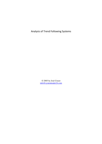
Analysis of Trend Following systemsLosing TradesLosing %Gross LossAvg LossAvg Loss %Avg Bars HeldMax ConsecutiveMax DrawdownMax Drawdown %Max Drawdown DateWealth‐Lab ScoreProfit FactorRecovery FactorPayoff RatioSharpe RatioUlcer IndexWealth‐Lab Error TermWealth‐Lab Reward RatioLuck CoefficientPessimistic Rate of ReturnEquity Drop Ratio31661.36% ‐26,002,824.58 ‐82,287.42‐5.88%43.851222360.60% ‐18,385,480.10 ‐82,446.10‐5.80%41.42129363.27% ‐7,617,344.48 ‐81,906.93‐6.06%49.6910 ‐5,631,295.00‐46.96%8/25/2004 ‐5,325,782.00‐75.77%8/27/2004 25.9725.670.226.380.800.98Stability test: Different lookback‐periods for moving averagesInitially, we used 50 and 100 as parameters for the SMA-periods. We now want to see what impactdifferent lookback periods have on our performance. Therefore, we run several simulations wherewe use different parameters in order to prove the system’s robustness. When doing this, we will usethe same parameter across all markets alike. Thus, we do not try to find the best parameter for everymarket separately. Although it is possible to design a system in Wealth Lab Developer using thebest parameter for each market we believe that this would mean to over optimize the system and itwould lead us into a curve-fitting-trap. If you search for (and later apply) the best parameter foreach market, the system might not be robust enough in the future and is likely to generate worseprofits than during your simulation.The simulation has been run for each parameter combination and the annualized profit has beenpainted in Figure 5. The different shading represents different annualized profit ratios (percentprofit per year). The vertical axis shows values for the fast SMA. The horizontal axis shows thedifference between the fast and the slow SMA. So, for example, the point at (50, 50) represents asimulation result using 50 as parameter for the fast SMA and 100 for the slow SMA.- 12 -
Analysis of Trend Following systemsFigure 5The graphic shows optimum values in the center of the chart. So, combinations of 40-60 for the fastSMA and 100-120 for the slow SMA provide the best results in backtesting.In our case, the optimum combination of (50, 60; i.e. SMAs of 50 and 110) is surrounded byparameter combinations with results of more than 12% p.a. So, this parameter combination is agood choice because slight changes in the market behavior provide still good results. We shouldexpect results in this magnitude if we use these parameters for our real trading.SMA Crossover weeklyAs our system tries to find long-term trends, we will now test if the usage of a weekly timescale issuitable, too. So, instead of computing our moving average points every day, we will use weeklySMAs which are calculated using the closing price of each week instead of the closing price of eachday. So, there will be only once a week (Friday evening) a possible crossover and therefore onlyonce a week (Monday morning) new orders have to be submitted to the broker. This makes tradingsuch a system much more comfortable. According to the initial system with SMA parameters of 50and 100 days, we will now use the weekly counterpart, i.e. 10 and 20 weeks of lookback periods.However, with our initial risk setting of 2% we are getting a low margin to equity ratio (exposure)of only 8.2%. Therefore, we allow an exception here and execute this test with 3% risk stop. Allother parameters remain the same.Rules:- Go Long the next day at Market ( on the Open) as soon as the fast SMA (of 10 weeks)crosses over the slow SMA (of 20 weeks)- Exit Long and Go Short the next day at Market as soon as the fast SMA (of 10 weeks)crosses under the slow SMA (of 20 weeks)- Set a StopLoss of 4 times the ATR (Average True Range*) of 10 weeksPosition sizing:3% based on initial stop loss (based on 4 times the 10-week-ATR)- 13 -
Analysis of Trend Following systemsExample trade:Figure 6 shows some example trades in Crude Oil. During 2003 the system experiences variouswhipsaws as the market changes its direction various times and no trend is established. But at theend of 2003, the system enters a long trade in which it stays until the end of 2004. Though it enterswhen the trend is already established it still catches 16 full points in this trade.Figure 6Results:Our portfolio equity curve (Figure 7) has a similar shape as the one of the daily system. However, itdoes not show the same (high) performance nor the same (high) drawdown. Still, the annualizedgain of over 11% is acceptable, especially taking the low number of trades into account (400 in 15years) which make this system easy to trade. Maximum drawdown is 38.6%, which is also lowerthan in the daily system. Please also note in the drawdown graph (Figure 8) that most drawdownsare below 10% whereas in the daily system (Figure 4) most are between 10% and 20%. Again, thissystem shows a low number of profitable trades (40%) with a high profit per trade of almost 15%.Exposure (12.4%) is still much lower than in case of the daily system (21.6%) and therefore,increasing the position size even further could be considered in order to improve profits. However,this will also result in higher drawdowns.- 14 -
Analysis of Trend Following systemsPortfolio Equity Curve:Figure 7Drawdown Curve:Figure 8Performance data:Starting CapitalEnding CapitalNet ProfitNet Profit %Annualized Gain %ExposureNumber of TradesAvg Profit/LossAvg Profit/Loss %Avg Bars HeldWinning TradesWinning %Gross ProfitAvg ProfitAvg Profit %Avg Bars HeldMax ConsecutiveLong ShortLong OnlyShort Only 1,000,000.00 5,080,527.63 4,080,527.63408.05%11.45%12.43% 1,000,000.00 4,701,566.13 3,701,566.13370.16%10.87%12.50% 1,000,000.00 1,378,961.63 378,961.6337.90%2.17%1.41%400 10,201.322.26%19.41380 9,740.962.21%19.2120 18,948.083.29%23.1516140.25% 10,118,227.49 62,846.1314.91%31.42715340.26% 9,555,140.84 62,451.9014.86%31.378840.00% 563,086.65 70,385.8315.85%32.503- 15 -
Analysis of Trend Following systemsLosing TradesLosing %Gross LossAvg LossAvg Loss %Avg Bars HeldMax Consecutive23959.75% ‐6,042,733.17 ‐25,283.40‐6.26%11.321422759.74% ‐5,858,608.18 ‐25,808.85‐6.32%11.02141260.00% ‐184,124.99 ‐15,343.75‐5.08%16.924Max DrawdownMax Drawdown %Max Drawdown Date ‐1,517,648.25‐38.60%4/8/2002 ‐1,507,480.38‐42.18%4/8/2002 .245.260.412.461.040.56Wealth‐Lab ScoreProfit FactorRecovery FactorPayoff RatioSharpe RatioUlcer IndexWealth‐Lab Error TermWealth‐Lab Reward RatioLuck CoefficientPessimistic Rate of ReturnEquity Drop RatioTrend with Pattern EntryThe following system combines trend following and countertrend concepts. It is called Trend withPattern Entry (TPE) and was first introduced by Dion Kurczek and Volker Knapp in the ActiveTrader Magazine in April 2003. The system’s main idea is that prices above the SMA indicate abull trend and prices below the SMA indicate a bear trend. Additionally, the system waits for ashort-term countertrend reaction to enter the market. If prices are above the SMA, the system waitsfor three consecutive down-days to enter long the next day. Consequently, if the price is below theSMA the system w
Analysis of Trend Following systems - 5 - Trend Following systems Among large hedge funds, Trend Following systems are very popular, maybe even the most used ones. The main reason for that is simple: They are able to support large amounts of equity. The larger a fund is the more difficult it becomes for this fund to enter and exit the market.File Size: 924KB