WIXLIB

time tk 2 , then the stock price Sk 2 is:(3)bk 1Sk 2 (2)ak 1(1)(2)(bk bk )2B0 (1 r)tk 2 (2) (3)bk akB0 (1 r)tk 2(19)Agent no 1’s wealth at time tk 2 is thus:(1)(1)(1)Wk 2 ak 2 Sk 2 bk(1)(2)bk(2)(bk bk )B0 (1 r)tk 2(20)Focusing on these two periods only and assuming the above sequence ofevents, having bought stocks at time tk 1 and kept them at time tk 2 makesa better strategy for agent no 1 than always owning bonds. Such a strategyindeed induces greater wealth:(1)bk(2)bk(1)(2)(1)(bk bk )B0 (1 r)tk 2 bk B0 (1 r)tk 2(21)From the replicator dynamics, an agent who experiences such a winningstrategy is more likely to own stocks in the future. As we will discuss later,there are other reasons why stocks might be attractive.Finally, to make sure that the discrete dynamic equations indeed provideprobabilities, that is to say:(i) k N : 0 p0,k 1(22)we impose on γ t the constraint:3Xγ t ((i)a0 ) M 1(23)i 1where M is an upper-bound for the discounted stock price. If tx denotesthe first time at which two agents own stocks, then M can be defined as(Montin, 2004): M max S0 , (i)i 1 b0P3(i)min{i a(i) 6 0} {ax }x11B0 (24)

3Stochastic equilibria“For dynamic economic models, an equilibrium (or steady state)is defined to be a point in the state space that is stationary underthe period to period transition rule. In the case of stochasticeconomies, a state cannot be stationary in the same sense as thatof deterministic models, given that shocks continue to disturbactivity in each period. Instead a steady state must be viewedas a situation where the probabilistic laws that govern the statevariables cease to change over time (Stachurski).”The state sk of the composite system at time tk is completely described bythe following random vector:(1)(2)(3)(1)(2)(3)(1)(2)(3)sk (xk , p0,k , p0,k , p0,k , ak , ak , ak , bk , bk , bk , Sk )(25)where xk equals A, B, C, D, E or F depending on the present configurationat time tk and Sk denotes the discounted stock price at time tk . Let’s callΣ the state space. By construction:Σ {a, · · · , F } [0, 1]3 [0,3X(i)a0 ]3 [0,i 13X(i)b0 ]3 [0, M ](26)i 1We consider the square metric ρ on the state space Σ:ρ(u, v) max{di (ui , vi )}i(27)The metric chosen for the first dimension induces the discrete topology:d1 (u1 , v1 ) 1 if u1 6 v1(28) 0 if u1 v1The usual distance on R is used for the other dimensions. We complete thestate space Σ with its limit points so that it is compact. Let Σ denote the12

Borel σ field of Σ.Agents face the following set of events:e1 configuration A is present at the following time step.e6 configuration F is present at the following time stepLet E {e1 , · · · , e6 } be the space of events and E be its power set.The stochastic kernel Q : Σ E [0, 1] gives the probability Q(s, A) ofrealizing the event A E given that the current state is s Σ.The mapping θ : Σ E Σ specifies which state succeeds: sk 1 θ(sk , ei ).We could write explicitly Q and θ (Montin, 2004). With the above definitions, it is easy to prove that our simplified economy is a random dynamicalsystem (Futia, 1982). As such, the function P : Σ Σ [0, 1] defined by:P (s, A) Q(s, (θ 1 A)s )(29)where (θ 1 A)s {e E θ(s, e) A} is the section of Imθ A determinedby s, is a transition probability. With our choice of state representation, ourdynamic economy is thus a discrete-time Markov process.The n step transition probability P n (s, A) is defined recursively:P 0 (s, A) 1if s A 0otherwiseP n (s, A) ZP n 1 (s, dt) P (t, A) (30)ΣLet B(Σ) denote the set of all bounded, Σ measurable, real-valued functions on Σ. B(Σ) is a Banach space under the sup norm: kf k sups Σ f (s) .The Markov operator associated to the transition probability P is the continuous linear transformation T : B(Σ) B(Σ) defined by:Z(T f )(s) f (t)P (s, dt)Σ13(31)

Notice that: kT k supkf k 1 kT f k 1.By isometric isomorphism (Dunford and Schwartz, 1957), we can define theadjointT : ba(Σ) ba(Σ) by: A Σ,(T λ)(A) ZP (s, A)λ(ds)(32)Σwhere ba(Σ) denotes the Banach space of all bounded finitely additive setfunctions λ under the total variation norm. Notice that T maps probabilities into probabilities.RMore generally, the nth iterate satisfies: [(T )n λ](A) Σ P n (s, A)λ(ds).By definition, an invariant probability measure λ, for a transition probability P , satisfies: A Σ :ZP (s, A)λ(ds) λ(A)(33)ΣIn other words, λ is a fixed point of the adjoint operator T .Our state space Σ being compact, the Markov operator T is tight. Moreover, T satisfies the Feller property, that is to say that T f is continuous andbounded whenever f is. We deduce from these two properties the existenceof at least one invariant probability measure λ. To reach stronger results,we adopt Canning’s key behavioral assumption (Canning, 1992):“Agents sometimes make mistakes, choosing an action that isindependent of their history. This condition implies that theempirical distribution of outcomes in the model converges to aunique limit distribution.”Allowing agents to make mistakes naturally makes our model more realisticas well. Notice that the word mistake could also encompass innovative14

strategies or overlapping generation models. At each time step:- with a probability p, agent no i makes a mistake and adopts the first(i)pure strategy with the initial probability I (i) p0,0 ,- with a probability (1 p), agent no i plays according to the probabilities obtained from the replicator dynamic equations.At this point, we need to enlarge the space of events to take into consideration possible mistakes. Let Tp denote the Markov operator when agentsmake mistakes. Using Doeblin’s condition, we can show that Tp is quasicompact.(1)Moreover, the state s (A, I (1) , I (2) , I (3) , 0, 0, a(3) , b(1) , b(2) , 0, ab (3) B0 ) satisfies the generalized uniqueness criterion: for any integer k 1, any states Σ and any neighborhood U of s, there exits an integer n such thatP nk (s, U ) 0.By allowing agents to make mistakes, we have given a special role to thestate s (and to other states of the same form). Indeed, if the composite system is in an arbitrary state sk at time tk , then the state s will be reached attime tk 3 with a strictly positive probability independent of sk . The proofsof the above two properties rely on this remark.From the above, we conclude that:- there exists a unique invariant probability measure λp ,- the sequence of probability measures {(Tp )n µ}, for any initial probability measure µ, converges to λp at a geometric rate in the topologyinduced by the total variation norm.In words, the unique invariant probability measure λp reflects the long runaverage (Cesaro sequence:1nPn ii 0 (Tp ) µ)15and the limit behavior for any ini-

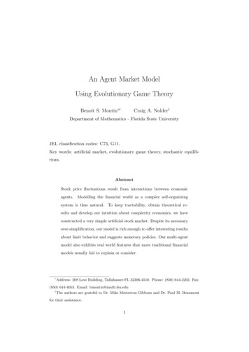
tial condition. Moreover, when the probability of making a mistake p tendsto zero, the equilibrium distribution λp converges to an invariant distributionλ for the model without mistakes. Formally, the equilibrium correspondenceE : p λp is upper hemi-continuous in the topology of weak convergence atp 0. Mistakes can thus be considered as an equilibrium selection device.However, as Canning (1992) warns us:“While mistakes are a refinement, they do not necessarily pickout a unique equilibrium; in some cases the distribution of themistakes, which actions are chosen if a mistake is made, mayaffect which equilibrium is selected.”Montin (2004) provides proofs of the properties of this section.4SimulationsAll simulations have been performed with Matlab.Simulated stock price fluctuations over one year (250 trading days) are plotted in figure 4. At each time step (for simplicity’s sake, tk k), a randomnumber generator is used to make the composite system collapse to an attainable configuration according to the transition probabilities.We have used the following set of parameters: S0 B0 1 (2) (1)(3)(1)(2)(3)a0 a0 0 a0 6 b0 4 b0 3 b0 0 p 0.02 (the probability of making a mistake) 1 r (1.1) 250 1 (the annual riskfree rate of interest is 10%)It is quite intuitive to understand that the stock’s high volatility comes fromits lack of liquidity. A model involving more agents would most probably lead16

to lower daily average returns and volatilities. The high historic annualizedSharpe ratio (approximately 2.09) gives a second explanation to why agentsmight like stocks.Figure 4: stock price fluctuationsAs a simple monetary policy, we now study the impact of a decrease ofthe riskfree rate of interest r on the limit distribution of the discountedstock price. Recall that the iterates {P n (s, .) (Tp )n δs } converge to theinvariant distribution λp at a geometric rate in the topology induced by thetotal variation norm. When agents make mistakes, there are 32 possiblesucceeding states sk 1 to sk . Exploring the entire tree to compute the exactdistribution after n iterations quickly becomes unrealistic. We thus adopta frequentist approach. Figure 5 represents the empirical distributions ofthe discounted stock price after respectively 200 and 250 iterations. Bothdistributions have been constructed with 15, 000 independent sample paths.To better visualize the impact of r, we have chosen the one-period riskfreerate to be equal to r 0.05. We have also computed the distance inducedby the total variation norm between the two distributions (d ' 0.11) to17

measure the quality of convergence toward the unique invariant distributionλp .Figure 5: discounted stock price distributions after 200 and 250 iterationsQualitatively, a decrease of the riskfree rate of interest r has two complementary consequences on the shape of the limit distribution of the discountedstock price.- As it can be observed in figure 6, positive rates of interest induce theexistence of local left-tails shifting the mean of the discounted stockprice to lower values. The larger the rate of interest is, the wider thelocal tails are.- Intuitively, decreasing the riskfree rate of interest r makes stocks moreattractive. From the replicator equations, it is easy to prove that the(i)probability p1,k , with which agent no i is willing to own stocks at timetk 1 , indeed increases when r decreases. It is thus more likely to be ina configuration of the second class (two agents own stocks) for lowervalues of r. Discounted stock price fluctuations resulting from transitions among configurations of the second class correspond to the right18

side of the discounted stock price distribution.Figure 6: discounted stock price distributions after 250 iterations for r 0.05, r 0.025, r 0.01 and r 0Finally, figure 7 gives the empirical distribution of the one-period stock logreturns after 250 iterations: ln S250S249 . The probability that the log returnequals zero is approximately 0.6664. To better visualize the tails of thedistribution, the y axis stops at the value 0.045. Again, the distributionhas been constructed with 15, 000 independent sample paths and the dailyrisk free rate of interest is 0.05. For comparison, the Gaussian distribution,with the same first two moments, is also represented. It is striking andcomforting that the empirical distribution’s peak around the mean is higher19

and narrower and that the tails are fatter (leptokurtic). This is a nice resultsince more traditional financial models usually fail to consider or explainsuch real world features (e.g., Pagan, 1996). The skewness and kurtosis are:Skewness ' 1.07Kurtosis ' 8.03The above values partially explain why agents might like stocks. The expected net stock return over one period is approximately 0.05, that is tosay very similar to the riskfree rate of interest r. But there are states ofthe world with very high payoffs. Friedman and Savage’s (1948) doubleinflection utility function could explain the agents’ behavior: depending onthe level of wealth, an agent is risk-averse (poor) or risk-loving (wealthy).Figure 7: log returns, Gaussian and hyperbolic distributionsThe class of generalized hyperbolic distributions exhibits the observed semi20

heavy-tails. The subclass of hyperbolic distributions was introduced in finance by Eberlein and Keller (1995). Their Lebesgue density can be expressed as:pdH (x) qα2 β 2pexp( αδ 2 (x µ)2 β(x µ))2αδK1 (δ α2 β 2 )(34)where K1 denotes the modified Bessel function of the third kind. The improvement in fitting our empirical log return distribution with an hyperbolicdistribution instead of a Gaussian distribution is as well illustrated in figure7. The parameters have been estimated by maximum likelihood with thefree statistical software R (we have also truncated the peak to better fit thetails).5ConclusionOther aspects, such as option pricing, can easily be studied in the frame ofour model. If only two agents were present, then our setting would fall underthe extensively studied Cox-Ross Rubinstein binomial tree (1979). Indeed,only two events could occur: the agents remain in their respective states orthey switch allocations. With three agents, given the stock price Sk at timetk , there are four possible values for Sk 1 . With two assets, it is not possibleto replicate an arbitrary contingent claim: the market is incomplete. Thepotential buyers and sellers have different goals and set different prices. Wecan follow Mel’nikov (1999) for an intuitive definition of the bid and askprices: To hedge the claim’s risk, the seller is ready to sell the claim for aprice equal to the most inexpensive portfolio that ensures a cashflowat maturity greater than or equal to the claim’s cashflow.21

Conversely, the buyer of the claim is ready to short-sell the most expensive portfolio which cashflow at maturity is covered by the claim’scashflow.The interested reader should refer to Mel’nikov (1999) and Montin (2004)for a more complete analysis with examples.Most agent-based computational economies heavily rely on simulations. Having adopted a simple representation of financial markets, we have been ableto prove theoretical results and gain intuition on complexity economics. Ofinterest, the limit empirical stock log return distribution presents real worldfeatures usually not taken into account by more traditional models. Wehope to create more realistic models as by-products of these first steps.22

References[1] Chiu Fan Lee and Neil F. Johnson, 2003. Efficiency and formalism ofquantum games. Physical Review A, 67 (2), reference 022311.[2] David Canning, 1992. Average behavior in learning models. Journal ofEconomic Theory, 57, 442-472.[3] Drew Fudenberg and David K. Levine, 1998. The Theory of Learningin Games. The MIT Press.[4] Larry Samuelson, 1997. Evolutionary Games and Equilibrium Selection.The MIT Press.[5] Benoı̂t Montin, 2004. A Stock Market Agent-Based Model Using Evolutionary Game Theory and Quantum Mechanical Formalism. PhD thesis, FSU.www.math.fsu.edu/ bmontin[6] John Stachurski. Lagrange stability in economic-systems with positiveinvariant density. Unpublished.[7] Carl A. Futia, 1982. Invariant distributions and the limiting behaviorof Markovian economic models. Econometrica, 50 (2), 377-408.[8] Nelson Dunford and Jacob T. Schwartz, 1957. Linear Operators (PartI). Interscience Publishers, New York.[9] Adrian Pagan, 1996. The econometrics of financial markets. Journal ofEmpirical Finance, 3 (1), 15-102.[10] Milton Friedman and Leonard Jimmie Savage, 1948. The utility analysisof choices involving risk. Journal of Political Economy, 56 (4), 279-304.23

[11] Ernst Eberlein and Ulrich Keller, 1995. Hyperbolic distributions in finance. Bernoulli, 1, 281-299.[12] John C. Cox, Stephen A. Ross and Mark Rubinstein, 1979. Optionpricing: a simplified approach. Journal of Financial Economics, 7 (3),229-263.[13] Alexander V. Mel’nikov, 1999. Financial Markets: Stochastic Analysisand the Pricing of Derivative Securities in: Translations of Mathematical Monographs, Vol. 184, American Mathematical Society.24

An Agent Market Model Using Evolutionary Game Theory Benoˆıt S. Montin † Craig A. Nolder† Department of Mathematics - Florida State University JEL classification codes: C73, G11. Key words: artificial market, evolutionary game theory, stochastic equilib-rium. Abstract Stock price