WIXLIB

8CHAPTER 11.2 Linear Equations in Linear AlgebraSOLUTIONSNotes: The key exercises are 1–20 and 23–28. (Students should work at least four or five from Exercises7–14, in preparation for Section 1.5.)1. Reduced echelon form: a and b. Echelon form: d. Not echelon: c.2. Reduced echelon form: a. Echelon form: b and d. Not echelon: c. 13. 4 6 14. 3 52573684 17 09 02 3 5 1 0 02103204 13 00 03577 19 01 03 4 8579 1 0 03105207 13 01 0 5. 0* , 0* 0,0 0 17. 3397 1 6 0473 6 100105 8 163104 1 9 0 15 0 12031 80 10 01 0010 6. 0 0 0 304 57 1 15 0Corresponding system of equations:4 3 15 32 10 2 3 . Pivot cols 1 and 2.0 7 1 12 0 34 052021 530x1 3x2x33100 Pivot cols0 .1, 2, and 41 * , 00 0412577 13 0 34 052 16 120 1 4 6* 00 , 00 07 1 3 04 7 9 368520 1 3 57 3 10 3557797 9 1 0 0 3001 5 3 5 3The basic variables (corresponding to the pivot positions) are x1 and x3. The remaining variable x2 is free.Solve for the basic variables in terms of the free variable. The general solution is x1 5 3x2 x2 is free x 3 3Note: Exercise 7 is paired with Exercise 10.

1.2 18. 2477 1 10 0004 17 1 4 000Corresponding system of equations:417 1 4 0000100 Solutions9 9 4 9 4x1x2The basic variables (corresponding to the pivot positions) are x1 and x2. The remaining variable x3 is free.Solve for the basic variables in terms of the free variable. In this particular problem, the basic variablesdo not depend on the value of the free variable. x1 9 General solution: x2 4 x is free 3Note: A common error in Exercise 8 is to assume that x3 is zero. To avoid this, identify the basic variablesfirst. Any remaining variables are free. (This type of computation will arise in Chapter 5.) 09. 11 2 675 1 6 0Corresponding system: 21x1x27 6 6 1 5 0 5 x3 4 6 x3 501 5 64 5 x1 4 5 x3 Basic variables: x1, x2; free variable: x3. General solution: x2 5 6 x3 x is free 3 110. 3 2 6 1 2 203 1 2 0Corresponding system:x1 113 1 7 0 2 x2 2001 4 7 4x3 7 x1 4 2 x2 Basic variables: x1, x3; free variable: x2. General solution: x2 is free x 7 3 311. 9 6 42128 6 40 30 00 0x1Corresponding system: 420000 4x230 10 00 0 4 / 32/300002x330 00 0 00 0 0

10CHAPTER 1 Linear Equations in Linear Algebra42 x1 3 x2 3 x3 Basic variable: x1; free variables x2, x3. General solution: x2 is free x is free 3 112. 0 1 706071 4 225 1 3 07 0x1 706001 4 28 7 x2x3Corresponding system:5 1 3 012 0 7060010 205 3 0 6 x4 5 2 x4 30 0 x1 5 7 x2 6 x4 x is free Basic variables: x1 and x3; free variables: x2, x4. General solution: 2 x3 3 2 x4 x4 is free 1 013. 0 0 31000000 1010 2 11 0 4 0 0 00 490 3100x1Corresponding system:x2x4000000109 490 3x5 5 4 x5 9 x5 1 42 11 0 4 0 0 0010000000 0 x1 5 3x5 x 1 4x5 2Basic variables: x1, x2, x4; free variables: x3, x5. General solution: x3 is free x 4 9x5 4 x5 is freeNote: The Study Guide discusses the common mistake x3 0. 1 014. 0 021 5 6 6 30000000010 5 12 0 0 0 0 0017 60 30000000010 9 2 0 0 0010 3 4905 1 4 0

1.2 7 x3x1Corresponding system:x2 6 x3 Solutions 9 3 x4 200 0x5 x1 9 7 x3 x 2 6 x 3x34 2Basic variables: x1, x2, x5; free variables: x3, x4. General solution: x3 is free x is free 4 x5 015. a. The system is consistent, with a unique solution.b. The system is inconsistent. (The rightmost column of the augmented matrix is a pivot column).16. a. The system is consistent, with a unique solution.b. The system is consistent. There are many solutions because x2 is a free variable. 217. 436h 2 7 030h The system has a solution only if 7 – 2h 0, that is, if h 7/2.7 2h 3 2 1 3 2 1 18. If h 15 is zero, that is, if h –15, then the system has no solution, h 7 0 h 153 5because 0 cannot equal 3. Otherwise, when h 15, the system has a solution.h2 1 h 2 119. 4 8 k 0 8 4h k 8 a. When h 2 and k 8, the augmented column is a pivot column, and the system is inconsistent.b. When h 2, the system is consistent and has a unique solution. There are no free variables.c. When h 2 and k 8, the system is consistent and has many solutions.32 1 3 2 120. 3 h k 0 h 9 k 6 a. When h 9 and k 6, the system is inconsistent, because the augmented column is a pivot column.b. When h 9, the system is consistent and has a unique solution. There are no free variables.c. When h 9 and k 6, the system is consistent and has many solutions.21. a.b.c.d.e.False. See Theorem 1.False. See the second paragraph of the section.True. Basic variables are defined after equation (4).True. This statement is at the beginning of Parametric Descriptions of Solution Sets.False. The row shown corresponds to the equation 5x4 0, which does not by itself lead to acontradiction. So the system might be consistent or it might be inconsistent.11

12CHAPTER 1 Linear Equations in Linear Algebra22. a. False. See the statement preceding Theorem 1. Only the reduced echelon form is unique.b. False. See the beginning of the subsection Pivot Positions. The pivot positions in a matrix aredetermined completely by the positions of the leading entries in the nonzero rows of any echelonform obtained from the matrix.c. True. See the paragraph after Example 3.d. False. The existence of at least one solution is not related to the presence or absence of free variables.If the system is inconsistent, the solution set is empty. See the solution of Practice Problem 2.e. True. See the paragraph just before Example 4.23. Yes. The system is consistent because with three pivots, there must be a pivot in the third (bottom) rowof the coefficient matrix. The reduced echelon form cannot contain a row of the form[0 0 0 0 0 1].24. The system is inconsistent because the pivot in column 5 means that there is a row of the form[0 0 0 0 1]. Since the matrix is the augmented matrix for a system, Theorem 2 shows that the systemhas no solution.25. If the coefficient matrix has a pivot position in every row, then there is a pivot position in the bottomrow, and there is no room for a pivot in the augmented column. So, the system is consistent, byTheorem 2.26. Since there are three pivots (one in each row), the augmented matrix must reduce to the formx1 a 1 0 0 a 0 1 0 b and so bx2 0 0 1 c x3 cNo matter what the values of a, b, and c, the solution exists and is unique.27. “If a linear system is consistent, then the solution is unique if and only if every column in the coefficientmatrix is a pivot column; otherwise there are infinitely many solutions. ”This statement is true because the free variables correspond to nonpivot columns of the coefficientmatrix. The columns are all pivot columns if and only if there are no free variables. And there are no freevariables if and only if the solution is unique, by Theorem 2.28. Every column in the augmented matrix except the rightmost column is a pivot column, and the rightmostcolumn is not a pivot column.29. An underdetermined system always has more variables than equations. There cannot be more basicvariables than there are equations, so there must be at least one free variable. Such a variable may beassigned infinitely many different values. If the system is consistent, each different value of a freevariable will produce a different solution.30. Example:x12 x1 x2 2 x2 x3 4 2 x3 531. Yes, a system of linear equations with more equations than unknowns can be consistent.x1 x2 2x2 0Example (in which x1 x2 1): x1 3x1 2 x2 5

1.2 Solutions1332. According to the numerical note in Section 1.2, when n 30 the reduction to echelon form takes about2(30)3/3 18,000 flops, while further reduction to reduced echelon form needs at most (30)2 900 flops.Of the total flops, the “backward phase” is about 900/18900 .048 or about 5%.When n 300, the estimates are 2(300)3/3 18,000,000 phase for the reduction to echelon form and(300)2 90,000 flops for the backward phase. The fraction associated with the backward phase is about(9 104) /(18 106) .005, or about .5%.33. For a quadratic polynomial p(t) a0 a1t a2t2 to exactly fit the data (1, 12), (2, 15), and (3, 16), thecoefficients a0, a1, a2 must satisfy the systems of equations given in the text. Row reduce the augmentedmatrix: 1 1 11 12 14 15 09 16 0123 1 0 01010011 12 133 084 011213 16 0 1 000100112 13 0 2 0111032 a4 0411103112 3 1 7 6 1 The polynomial is p(t) 7 6t – t2.34. [M] The system of equations to be solved is:a0 a1 0 a2 0 2 a3 032 a3 23 a3 43 3a0 a1 2 a2 2a0 a1 4 a2 42 2a0 a1 6a1 8a2 6 a2 82a0 a0 a1 10 a2 102 a3 63a3 8 a3 103 a5 05 a4 24 a5 25 2.90 a4 44 a5 45 14.8 a4 64 5 39.6a4 845 74.3 a4 104a5 6 a5 8 a5 105 0119The unknowns are a0, a1, , a5. Use technology to compute the reduced echelon of the augmentedmatrix: 1 0 1 2 1 4 1 6 1 8 1 10 1 0 0 0 0 80032960480026880902400 12.9 0 14.8 0 39.6 074.3 0 119 00 12.9 0 9 0 3.9 08.7 0 14.5 92003296048007680422400 2.9 9 30.9 62.7 104.5 0 2.9 9 3.9 6.9 24.5

14CHAPTER 1 Linear Equations in Linear Algebra 1 0 0 0 0 40 1 0 0 0 0 00200000480000848480001622457638400000010 12.9 0 9 0 3.9 0 6.9 0 10 0020000048000084848000 1 02.8167 06.5000 " 8.6000 0 0 26.900 .002604 0010000001000016224576384000010000001000 322.9 9609 48003.9 7680 6.9 1 .0026 0000010 1.7125 1.1948 .6615 .0701 .0026 Thus p(t) 1.7125t – 1.1948t2 .6615t3 – .0701t4 .0026t5, and p(7.5) 64.6 hundred lb.Notes: In Exercise 34, if the coefficients are retained to higher accuracy than shown here, then p(7.5) 64.8.If a polynomial of lower degree is used, the resulting system of equations is overdetermined. The augmentedmatrix for such a system is the same as the one used to find p, except that at least column 6 is missing. Whenthe augmented matrix is row reduced, the sixth row of the augmented matrix will be entirely zero except for anonzero entry in the augmented column, indicating that no solution exists.Exercise 34 requires 25 row operations. It should give students an appreciation for higher-levelcommands such as gauss and bgauss, discussed in Section 1.4 of the Study Guide. The command ref(reduced echelon form) is available, but I recommend postponing that command until Chapter 2.The Study Guide includes a “Mathematical Note” about the phrase, “If and only if,” used in Theorem 2.1.3SOLUTIONSNotes: The key exercises are 11–14, 17–22, 25, and 26. A discussion of Exercise 25 will help studentsunderstand the notation [a1 a2 a3], {a1, a2, a3}, and Span{a1, a2, a3}. 1 3 1 ( 3) 4 1. u v . 2 1 2 ( 1) 1 Using the definitions carefully, 1 3 1 ( 2)( 3) 1 6 5 u 2 v ( 2) , or, more quickly, 2 1 2 ( 2)( 1) 2 2 4 1 3 1 6 5 u 2v 2 . The intermediate step is often not written. 2 1 2 2 4 3 2 3 2 5 2. u v . 2 1 2 ( 1) 1 Using the definitions carefully,

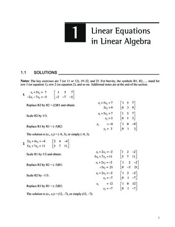
1.3 Solutions 3 2 3 ( 2)(2) 3 ( 4) 1 u 2 v ( 2) , or, more quickly, 2 1 2 ( 2)( 1) 2 2 4 3 2 3 4 1 u 2v 2 . The intermediate step is often not written. 2 1 2 2 4 3.x2u – 2vu–vu– 2vu v–vx1v4.u – 2vx2u–vu– 2vu v–vx1v 6 x1 3 x2 1 6 3 1 5. x1 1 x2 4 7 , x1 4 x2 7 , 5 x1 0 5 5 0 5 6 x1 3x2 1 x1 4 x2 75 x1 5 6 x1 3x2 1 x 4 x 7 2 1 5 x1 5 Usually the intermediate steps are not displayed. 2 8 1 0 6. x1 x2 x3 , 3 5 6 0 2 x2 8 x2 x3 3x1 5 x2 6 x3 2 x1 8 x2 x3 0 , 3x1 5 x2 6 x3 0 00 2 x1 8 x2 x3 0 3 x 5 x 6 x 0 23 1Usually the intermediate steps are not displayed.7. See the figure below. Since the grid can be extended in every direction, the figure suggests that everyvector in R2 can be written as a linear combination of u and v.To write a vector a as a linear combination of u and v, imagine walking from the origin to a along thegrid "streets" and keep track of how many "blocks" you travel in the u-direction and how many in thev-direction.a. To reach a from the origin, you might travel 1 unit in the u-direction and –2 units in the v-direction(that is, 2 units in the negative v-direction). Hence a u – 2v.15

16CHAPTER 1 Linear Equations in Linear Algebrab. To reach b from the origin, travel 2 units in the u-direction and –2 units in the v-direction. Sob 2u – 2v. Or, use the fact that b is 1 unit in the u-direction from a, so thatb a u (u – 2v) u 2u – 2vc. The vector c is –1.5 units from b in the v-direction, soc b – 1.5v (2u – 2v) – 1.5v 2u – 3.5vd. The “map” suggests that you can reach d if you travel 3 units in the u-direction and –4 units in thev-direction. If you prefer to stay on the paths displayed on the map, you might travel from the originto –3v, then move 3 units in the u-direction, and finally move –1 unit in the v-direction. Sod –3v 3u – v 3u – 4vAnother solution isd b – 2v u (2u – 2v) – 2v u 3u – 4vdbcu2vva0w–v–2vy–uxzFigure for Exercises 7 and 88. See the figure above. Since the grid can be extended in every direction, the figure suggests that everyvector in R2 can be written as a linear combination of u and v.w. To reach w from the origin, travel –1 units in the u-direction (that is, 1 unit in the negativeu-direction) and travel 2 units in the v-direction. Thus, w (–1)u 2v, or w 2v – u.x. To reach x from the origin, travel 2 units in the v-direction and –2 units in the u-direction. Thus,x –2u 2v. Or, use the fact that x is –1 units in the u-direction from w, so thatx w – u (–u 2v) – u –2u 2vy. The vector y is 1.5 units from x in the v-direction, soy x 1.5v (–2u 2v) 1.5v –2u 3.5vz. The map suggests that you can reach z if you travel 4 units in the v-direction and –3 units in theu-direction. So z 4v – 3u –3u 4v. If you prefer to stay on the paths displayed on the “map,” youmight travel from the origin to –2u, then 4 units in the v-direction, and finally move –1 unit inthe u-direction. Soz –2u 4v – u –3u 4v9. 4 x1 x1x2 6 x2 3x2 5 x3 x3 8 x3 0 0, 0 0 x2 5 x3 0 4 x 6 x x 0 ,3 1 2 x1 3 x2 8 x3 0 x2 5 x3 0 4 x 6 x x 0 23 1 x1 3 x2 8 x3 0 0 1 5 0 x1 4 x2 6 x3 1 0 1 3 8 0 Usually, the intermediate calculations are not displayed.

1.3 Solutions17Note: The Study Guide says, “Check with your instructor whether you need to “show work” on a problemsuch as Exercise 9.” 9 2 , 15 4 x1 x2 3 x3 9 x 7x 2x 2 23 1 8 x1 6 x2 5 x3 15 4 x1 x2 3x3 9 x1 7 x2 2 x3 2 , 8 x1 6 x2 5 x3 15 4 1 3 9 x1 1 x2 7 x3 2 2 8 6 5 15 4 x110. x18 x1 x2 7 x2 6 x2 3x3 2 x3 5 x3Usually, the intermediate calculations are not displayed.11. The questionIs b a linear combination of a1, a2, and a3?is equivalent to the questionDoes the vector equation x1a1 x2a2 x3a3 b have a solution?The equation 1 0 5 2 x1 2 x2 1 x3 6 1 0 2 8 6 a1a2a3(*)bhas the same solution set as the linear system whose augmented matrix is52 1 0 M 2 1 6 1 0 286 Row reduce M until the pivot positions are visible: 1 0 5 2 1 0 5 2 M 0 1 4 3 0 1 4 3 0 2 8 6 0 0 0 0 The linear system corresponding to M has a solution, so the vector equation (*) has a solution, andtherefore b is a linear combination of a1, a2, and a3.12. The equation 1 0 2 5 x1 2 x2 5 x3 0 11 2 5 8 7 a1a2a3bhas the same solution set as the linear system whose augmented matrix is(*)

18CHAPTER 1 Linear Equations in Linear Algebra 1 0 2 5 M 2 5 0 11 2 5 8 7 Row reduce M until the pivot positions are visible: 1 0 2 5 1 0 2 5 M 0 5 41 0 5 41 0 5 43 0 0 02 The linear system corresponding to M has no solution, so the vector equation (*) has no solution, andtherefore b is not a linear combination of a1, a2, and a3.13. Denote the columns o

2 CHAPTER 1 Linear Equations in Linear Algebra 3. The point of intersection satisfies the system of two linear equations: . See the remarks following the box titled Elementary Row Operations. b. False. A 5 6 matrix has five rows. c. False. The description given applied to a single solution. The solution set consists of all possible