WIXLIB

Fig. 3.Average Points Per Game Per Team Over 82 Gameskept changing until the end of the season.2 When we trainedonly on the running averages in the 1st half of the season andtested on the running averages in the 2nd half of the season,we managed a get a test accuracy of 66%.The next step we tried from this was using SVMs toclassify the game as win or loss.IV.S UPPORT V ECTOR M ACHINEUsing the full game data from the database, implementeda support vector machine model to classify each game sampleas a binary variable 1 (win) or 0 (loss). We used the SVM inconjunction with a lasso regression and bootstrap aggregatingto achieve our final prediction. Before implementing the algorithm, we pre-processed the raw data was had scaled andcalculated the average of various team statistics from eachseason (rebounds per game, points per game, etc.). Further,for each game we created a sample point with the averagesfor both teams as features.Even in this reduced form there were still 79 variablesfeatures. To infer which of the predictors were most significantwe ran a lasso regression on the data. The lasso, a type ofshrinkage regression, set several of our predictors coefficientsto zero, which justified their exclusion from our model becausethey were insignificant. Our lasso model was tested over arange of shrinkage parameters and was then 10-fold crossvalidated. We chose the best model after cross validation toselect our best subset of predictors. Though the data for ourlasso model was of varied size and character throughout ourexperimental trials, the lasso generally left approximately 20predictor coefficients nonzero.Using the set of predictors that had been found to be mostsignificant, we fit a polynomial kernel support vector classifierto the data. We implemented the SVM and tuned the result tofind the optimal cost parameter and polynomial degree froma range using simple cross validation. This model was ableto predict the win response for whole seasons of games with2 If you look at Indiana’s steady increase in average points per game, it canbe attributed to Paul George’s meteoric growth as a player. Our models neveraccount for player or team growth.accuracy in the range of 65-69%.To further optimize the prediction of the SVM we alsoimplemented bootstrap aggregating (bagging) over the SVMlasso model. We bootstrapped over our entire model so that thelasso would be fit onto each bootstrap re-sample and decidewhich sample were significant in that bootstrap set. Then we fitthe SVM to the re-sample and predicted the results for the testset. Averaging the predictions over 20 bootstrap re-samples,we set the sample with an average of less than .5 to 0 and therest to 1. In the best case we were able to bag over a modeltrained on the 2012-13 season and predict the results of the2011-12 season with 68.4% accuracy and the results of the2010-11 season with 65.1% accuracy.We also explored fitting the model on a larger trainingset, which led too a small improvement in test accuracy. Wefitted and bagged a model trained on the 2010-11 and 2011-12seasons and predicted the 2012-13 results with 68.9% accuracy. This was our best non-training error from the lasso/SVMmodel. This is a strong result in context; ESPNs Accuscorealgorithm for NBA odds (win/loss) bets had an accuracy of70.3% last season. Though a consistent expert picks panel doesnot formally exist at ESPN for basketball, in NFL football theAccuscore football equivalent has been more accurate than anyESPN expert for the past 3 years.To examine the real effect of our model we calculatedthe real-time average of a teams statistics for the 2012-13season and ran our bagged lasso/SVM model on a trainingset that used the previous two seasons as well as an arbitrarynumber of elapsed games in the 2012-13 season. When wepredicted the remain games of the season we consistentlyachieved accuracies of 63.5% (70% of games remaining) orgreater with the accuracy increasing to 65.6% toward the endof the season (30% of games remaining). We also ran thepredictor on the entire running averages set and got an accuracyof 65%. Though this test of the true use-case yielded weakerresults than the full-season retrospective classifications, webelieve that given more time we could improve the model.First, we could calculate running averages for each seasonand use these samples to train the data. We could also goa level deeper in detail and try to use a construction of playerstatistic contributions (in real season time) to construct theteam average statistics and then make predictions.A. BoostingOne of the methods cited by TeamRankings.com as anelement of their prediction formula was a decision tree.Because of his success we also pursued a decision tree totry to classify our data. However, instead of simply fitting adecision tree regression to the data we implemented a Boostingmethod to combine a myriad of weak learner decision treesto form a strong learner tree at the end. We optimized bysimple cross validation over three different tuning parameters:the depth of the tree, the number of trees, and the shrinkageparameter lambda. Unfortunately, the accuracy of the modelplateaued at 64.5%. Boosting is a particularly slow and computationally heavy method so it was difficult to run a crossvalidations/optimizations over many combinations of depth,tree count, and shrinkage parameter.

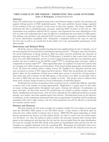
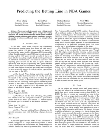
B. Spread and Over/Under AnalysisWe ended up developing full models to predict the spread,but to give us an initial idea on how spread and over/underlines are set, we ran a simple regression using teams averagesas predictors and the following graphs are the result.normalized statistics, we use polynomial regression along withSVM and Naive Bayes techniques to further enhance themodel’s predictions. The following steps describe the fullmethod we devised. Running this algorithm over a seasonAlgorithm 1 Calculate Time-Varying Defensive and OffensiveStrengths By Win PropagationRequire: λ, KO , KDOS (0) 1DS (0) 1for all game allGames dom numberOf GamesW innerHasP layedp numberOf GamesLoserHasP layed(m 1)(p)(m)OSwinner λOSwinner (1 λ)KO(m 1)(m)DSloser(m)OSwinner(p)OSloserD(m)DSwinner(m) 1 DSwinnerD OS (p)loser(m) 1 OSwinnerO DS (p)loserDSwinner λDSwinner (1 λ)K(p 1)(p)(p 1)(p)Fig. 4. Prediction of Spread and Over/Under using Basic Linear RegressionOSloser λOSloser (1 λ)KFrom the graphs, we can see a clear linear relationshipbetween what we predicted and what the final betting lineswere set at. The variance could come from betting housesadjusting to how the public is betting or variation in the modelsthat our linear model did not account for (such as injuredplayers, fatigue, etc). We then looked at how the Vegas spreadand over/under lines compared to actual game results.DSloser λDSloser (1 λ)KFig. 5.Spread and Over/Under vs. Actual Game ResultsFrom these graphs, it is clear that from the cloud shapethat there is a lot of noise in the actual games compared tothe predictions. This could be the underlying nature of sportsthat sports are inherently very noisy and there is nothing wecan do. On the other hand, the betting lines do a good jobsplitting their predictions in half, essentially meaning that theydo a good job themselves over the course of the season settingthe lines such that they are guaranteed to win.V.C AUSAL W EIGHTED R EGRESSIONIn our final approach, we attempted to create a model thatcaptures both the natural fluctuations in a team’s performancethroughout the season, and also adjust their statistics to moreaccurately reflect their performance in a game. For instance,a team that puts up a lot of points against the best teamin the league should potentially have their rating increased,even if they lose. We introduce the causal limitation somewhatartificially to this method, although our reasoning stems fromthe fact that we have a time-varying model, and it would notmake sense to incorporate future data. One thing to note isthat this is a hybrid approach, and once we obtain the causallyend forwill produce an estimated offensive strength (OS ( m)) and adefensive strength(DS ( m)) where m M gamesperseasonis the number of games played for each team. The constantsKO and KD control the relative weighting of defense vs.offense, and λ is the forgetting factor - i.e. how much pastgame results should affect the current strengths. These valuesare then smoothed with a polynomial interpolator to get anestimate of a team’s offensive and defensive strengths relativeto the other teams at any point in the season. One importantthing to note is that we do withhold the test set from thetraining set when we apply the smoothing, as failure towithhold this data would cause the test data to leak into to thetraining data. The estimations of this method provide a fairlydecent relative representation of all the teams’ capabilities,at least when compared retrospectively to their performanceslast year. The defensive strengths of a team are then used inFig. 6. In the 2012 season, the Miami Heat were regarded as the bestdefensive team in the league. The Los Angeles Lakers were more or less inthe middle of the league both offensively and defensively.every game to normalize their stats to get an estimation oftheir effective stats relative to the league at that point. Thesevalues are similarly smoothed to reduce the high variance thatis inherent in sports data.These normalized statistics are then used in a linear regression over the training set to map a given statistic tonormalized points scored in a game. We found that a derivedstatistic called ”effective field goal percentage” (eFGP) was themost highly correlated with points scored, and so our modeluses only the regression fitted to this statistic in predictingthe normalized number of points that will be scored. Once

a normalized point prediction is made based on a teamssmoothed normalized eFGP going into a game, the predictionis de-normalized with the opposing teams estimated defensive(numGamesOpponentHasP layed)strength (DSopponent) to get a real scoreprediction. We can then compare the predicted scores for eachteam to get a predicted spread, and by comparing this to thegiven spread for the game, we are able to bet one way oranother.allows for better estimation of a team’s true value at anygiven time. We think that expanding upon the existing causalweighting algorithm to include more variables would significantly improve the strength estimation aspect of the model.It was disappointing that incorporating the extra classificationstep did not significantly improve the model, but given thatour predictions are hovering at around 50% anyway, it isnot surprising that the predictions have only a very smallcorrelation with the outcomes (if any), and no amount ofclassification can fix that.VI.Fig. 7. This regression is fitted for each team in the hopes of capturing anydiffering offensive paradigms between teams.To further improve our model’s ability to beat the spread,we incorporate both SVM and Naive Bayes classifiers trainedon a feature set of the game statistics in addition to ourpredictions. The classifiers are used both to directly predictwhether or not a team will beat the spread in a given game,and also to predict whether or not the prediction given bythe model will succeed or not. The first case is referred to asMethod 1, and the second as Method 2. Here are the results ofthe model under various test schemes: K-fold Cross Validationwith K 10, and Random Holdout Cross Validation with30% of the data withheld as the test set. The RHCV values areobtained as the mean of 30 iterations. Though the above figuresTABLE IV.MethodNormal PredictorSVM Method 1SVM Method 2NB Method 1NB Method 2S PREAD P REDICTION M ODEL R ESULTS10-fold CV i52.53%51.69%52.78%51.42%51.10%10-fold CV ii51.67%50.84%50.84%50.52%51.22%30 RHCV i51.39%49.88%50.33%50.07%50.42%30 RHCV ii50.71%50.23%49.59%49.74%50.33%seem to imply that this would be a reasonable approach, ourresults show that it was not any more successful at predictinggame outcomes than the brute-force bulk approaches discussedearlier (win/loss prediction results not shown in table as theyhave been discussed at length in prior sections). However,since this model was designed specifically with the goal ofpredicting the point spread, it is not surprising that it wouldperform worse with regard to winner prediction. Beating thespread is not necessarily the same problem as predicting thewinning team. We also tested this model under more stringentconditions imposed due its causal nature, so this probablyaccounts for the lower performance in win/loss predictionaccuracy. With our results, we are reluctant to believe thatour model achieves significantly better than 50% predictionaccuracy vs. the spread, and although multiple iterations ofthe two cross-validation schemes did show a slight favorableedge towards 51% and 52%, we are certainly not beatingthe requisite 52.4% prediction accuracy required to enact afinancially rewarding betting strategy.This modeling approach makes more rigid assumptionsabout the time-varying nature of team performance, but alsoC ONCLUSIONIn this report we have shown that machine learning techniques can be successfully applied to NBA games to predictthe winner of any given game with around 68% accuracy.This level of accuracy rivals that of professional analysts andbasketball experts. However, in our endeavor to predict thespread outcomes with an accuracy greater than 52.4%, themodel we developed fails to meet this goal under testing.3There are several contributing factors to this.Once our model was trained, it resulted in a simpledeterministic predictor. Ideally, since we are trying to modelthe interactions of complex entities, we would like to add morelayers to our model and incorporate an element of stochasticity.This in conjunction with batch simulation would probablyconverge on a more accurate estimate for game outcomes thanour train-once, predict-once method. Successful sports bettingcompanies such as Accuscore claim to use this batch simulation approach. Implementation of a more complex stochasticmodel would require greater access to specialized data, andalso more computational power to run many simulations. Theseare limitations that an individual wishing to beat the spreadwill always face, and it is no surprise that the predictors withmore resources at their disposal are able to perform better.We conclude that in order to make predictions about such acomplex interaction, the quality and complexity of the dataused is perhaps the most important factor in determining thesuccess of the model.ACKNOWLEDGMENTThe members of this project team would like to thankAndrew Ng and his teaching staff for sharing their wealth ofknowledge on the related subject material. We should also liketo thank Yuki Yanase for helping manually collect betting datafrom the ESPN website.R EFERENCES[1][2][3][4][5]Adams M, Ryan P., George E. Dahl, and Iain Murray. ”IncorporatingSide Information in Probabilistic Matrix Factorization with GaussianProcesses.” 25 Mar, 2010. arxiv.org.”Four Factors.” Basketball Reference. n.d. basketball-reference.com.Hess, David. ”Under the TeamRankings Hood, Part 4: Models, Models,Everywhere.” TeamRankings. 12 Mar, 2011. teamrankings.com.Shi, Zifan et al. ”Predicting NCAAB match outcomes using ML techniques - some results and lessons learned.” 14 Oct, 2013. arxiv.org.Walsh, PJ. ”How to bet over/unders.” ESPN Insider. 4 Dec, 2013.insider.espn.go.com.3 For the poster presentation, we made a prediction for that nightthat Orlando would beat the spread in their game against Charlotte. Wejust wanted to say, that our prediction was right: ORL 92 CHA 83 http://espn.go.com/nba/recap?gameId 400489191

the histogram of points scored per game. We see that this is a Fig. 1. Distribution of Points Scored Per Game for All Teams in NBA (2012-13) nearly perfect Gaussian distribution. Further, by breaking this down per team per year, we can see similar results with smaller datasets. For most of our tests, we make the assumption that the