Transcription
Multifactor Poisson and Gamma-Poisson models for callcenter arrival timesLawrence Brown and Linda Zhao1Department of StatisticsUniversity of PennsylvaniaHaipeng ShenDepartment of Statistics and Operations ResearchUniversity of North Carolina at Chapel HillAvishai MandelaumDepartment of Industrial Engineering and ManagementTechnion UniversityDraftJanuary 26, 20041 Researchsupported in part by NSF grant and the Wharton Financial Institutions Center.
AbstractIt is usually assumed that the arrivals to a queue will follow a Poisson process. In itssimplest form, such a process has a constant arrival rate. However this assumption is notalways valid in practice. We develop statistical procedures to test a stochastic process is aninhomogeneous Poisson process, and show that call arrivals to a real-life call center followsuch a Poisson process with an inhomogeneous arrival rate over time. We find that theinhomogeneous Poisson assumption is reasonably well satisfied. Then we derive statisticalmodels that can be used to construct predictions of the inhomogeneous arrival rate, andprovide estimates of the parameters in the models. The conclusion that the process is wellmodelled as an inhomogeneous Poisson process, together with a statistical model for thearrival rate in that process, could be used to enable realistic calculations or simulations ofthe performance of the queuing system. The models can also be used to predict future callvolumes or workloads to the system.
1IntroductionCall centers allow groups of agents to serve customers remotely via the telephone. They havebecome a primary contact point between customers and their service providers and, as such,play an increasingly significant role in more developed economies. While call centers aretechnology-intensive operations, often 70% or more of their operating costs are devoted tohuman resources, and to minimize costs their managers carefully track and seek to maximizeagent utilization. Well-run call centers adhere to a sharply-defined balance between agentefficiency (measured by utilization level) and service quality (measured by the waiting timeof calls). To achieve the balance, they use queueing-theoretic models. One of the key inputsto these mathematical models is the rate at which call arrives. As noted in Jongbloed andKoole (2001) and Gans, Koole and Mandelbaum (2003), uncertainty in call volumes is oneof the main problems in managing a call center.In this article we propose to model the arrival process to a call center as an inhomogeneousPoisson process. A testing procedure is also developed to verify the proposal. The processhas a underlying smoothly varying rate function, λ, which depends on some covariates inthe data like date, time of day, type and priority of the calls.To make things a little complicated, the rate function λ is a hidden function that isnot observed. That is, λ is not functionally determined by date, time of day and call-typeinformation. This phenomenon is also observed before by Jongbloed and Koole (2001).Due to this feature, we develop models to predict statistically the number of arrivals as afunction of only those repetitive features. The methods also allows us to construct confidenceor prediction bounds in addition to predictions of future call volumes.Call-arrival data gathered at an Israeli call center is used as motivation and illustrationof the various problems and methodologies we discuss. We provide a very brief discussion inSection 2 of this data application.1
The rest of the paper is organized as follows. In Section 2 we describe the call centerdata we will use as an example of an application of our methodology. Section 3 proposesa methodology to test whether a stochastic process can be modelled as an inhomogeneousPoisson process. The method is also illustrated on the Israeli call center data. After verifyingthe call arrival process is an inhomogeneous Poisson process, Section 4 introduces threedifferent models to estimate the underlying Poisson arrival rate. The models can also beused to predict future call volumes. We conclude this article with a case study in Section5, where our proposed tests and models are illustrated on arrival data from an Israeli callcenter.2Call Center Arrival DataThe data accompanying our study was gathered at a relatively small Israeli bank telephonecall center in 1999. The portion of the data of interest to us here involves records of thearrival time of service-request calls to the center. These are calls in which the caller requestsservice from a call center representative. It is reasonable to conjecture that these arrival timesare well modelled by an inhomogeneous Poisson process, as we will verify later in Section 3.The arrival rate for this process should depend on time of day, and perhaps other calendarrelated covariates such as month or day of the week. There are different categories of servicethat may be requested, and preliminary analysis clearly shows that this factor should alsobe considered since the arrival rate patterns differ considerably. For more information aboutvarious aspects of this data see Mandelbaum, Sakov and Zeltyn (2000). Different features ofthe data are investigated rather broadly by Brown, Gans, Mandelbaum, Sakov, Shen, Zeltynand Zhao (2003).2
3Arrivals are inhomogeneous PoissonComments from Haipeng: We would like to describe a procedure that one canuse to show a stochastic process is a Poisson process. To achieve that, we firstshow the arrivals do not depend on the exact time clock, then the arrivals areshown to be independent with each other. Finally we show that the inter-arrivaltimes are exponentially distributed. The procedure is illustrated using the Israelidata.Finally I added a section to show how the Poisson arrival rates are not easily“predictable”, to motivate the notion of modelling the arrival rates randomly.Basically this section was in our JASA paper, but was took out due to the lengthrequirements.Classical theoretical models posit that arrivals form a Poisson process. It is well knownthat such a process results from the following behavior: there exist many potential, statistically identical callers to the call center; there is a very small yet non-negligible probabilityfor each of them calling at any given minute, say, so that the average number of calls arrivingwithin a minute is moderate; and callers decide whether or not to call independently of eachother.Common call-center practice assumes that the arrival process is Poisson with a rate thatremains constant for blocks of time, often individual quarter-hours, half-hours or hours. Acall center manager will then fit a separate queueing model for each block of time, andestimated performance measures may shift abruptly from one interval to the next.A more natural model for capturing both stochastic and operational levels of detail isa time inhomogeneous Poisson process. Such a process is the result of time-varying probabilities that individual customers call, and it is completely characterized by its arrival-ratefunction λ. Knowledge that the arrivals follow an inhomogeneous Poisson process will be3
of use if it turns out that the arrival rate varies relatively slowly in time. Smooth variationof this sort is familiar in both theory and practice in a wide variety of contexts, and seemsreasonable in call centers.To be precise, we define an inhomogeneous Poisson process on [0, ) as follows. Lett [0, ). Let λ(t) denote the arrival rate, assumed continuous for simplicity, and letRtΛ(t) 0 λ(τ )dτ . Let ν(t) denote the cumulative count process for a standard Poissonprocess with arrival rate 1. Thus P {ν(t) k} e k /k! P oiss(k; 1). Then thecumulative number of counts for the inhomogeneous process is N (t) ν(Λ(t)). If λ(t) isapproximately a constant, λ, over some interval, say (a, b) then N (b) N (a) P oiss(·, λ).The assumption that N is such a process can thus be tested by looking at short time intervals,estimating λ over the interval, and testing whether N (t) follows a Poisson process law withconstant rate λ over the interval. The constant, λ, in this description may depend on theinterval.We construct below two tests of call center arrival processes designed to determinewhether the process is inhomogeneous Poisson with such a slowly varying arrival rate.3.1Testing no time dependenceOur first test is intended to discover whether there may be dependence on the exact clocktime within a given short clock interval over a period of many days. (There seems no a-priorireason why such dependence should exist in our data; it might in principle occur if severalcustomers had automatic phone systems designed to call the bank at the same time on everyday.) Choose a given relatively short time interval over which λ(t) can be presumed nearlyconstant on any given day. If λ(t) λdate is a constant over this interval on each day,then the counts within this time interval over many days will be (approximately) uniformlydistributed as a function of the clock time. This leads to a test of the null hypothesis.4
We illustrate this test by analyzing arrivals on regular workdays from 8/1 through 12/31during the time interval from 11:15 am to 11:30 am. (We have chosen for relatively arbitraryreasons to analyze only this 5-month period, rather than the whole year. Analysis of theentire year’s data yielded qualitatively similar results.)There were 3544 calls arriving to the queue during this period on such days. The histogram of these calls as a function of arrival time is shown in Figure 1.11.2511.311.3511.411.4511.5Figure 1: Histogram of call arrival time, for regular weekday calls from 8/1 through 12/31between 11:15am and 11:30am. (Time is indicated in decimals of an hour, so 11.25 11 :15am.)This histogram has a roughly uniform appearance. Standard tests of uniformity can beapplied to this data. For example, the Chi-squared test of uniformity based on the 30 binsshown in the histogram is based onχ2 X (observed bin count expected bin count)2expected bin count,where expected bin count 3544/30. This test statistic has 29 df under the null hypothesis.For the data shown in Figure 1 we computed χ2 26.4 and P-value .60.5
Alternatively, one could apply a one-sample Kolmogorov-Smirnov test of uniformity,based on the statistic ³ KS supn F̂n (t) F (t) ,where F̂n denotes the sample cumulative distribution function. For the data shown in Figure1 we computed KS 0.6727 and P-value 0.5.We computed similar χ2 and K-S tests for other 15-minute and 5-minute intervals. Mostwere not significant, as above. A few showed modestly significant results, with the mostnoticeable of these being for the interval from 2pm to 2:15pm, which had a χ2 value of 57.3on 29 df (P-value 0.001) and a similarly significant K-S value.For the sake of completeness, Figure 2 shows the histogram for the data between 2pmand 2:15pm. As far as we can see there is no special pattern here to describe the deviationsfrom the assumed uniformity of the null hypothesis:1414.114.2Figure 2: Histogram of call arrival time, for regular weekday calls from 8/1 through 12/31between 2pm and 2:15pm. (Time is indicated in decimals of an hour, so 14.1 2:06pm.)6
3.2Testing no serial dependenceComments from Haipeng: Are we trying to establish the independence of thearrival times here? If so, can we achieve that by showing the various transformations of the inter-arrival times are uncorrelated? I tried to put in some wordsbelow. Please feel free to modify.Another possible violation of the Poisson process assumption would involve dependenceamong the call arrival times. We can establish the independence by looking at correlationsof various transformations of the inter-arrival times.3.3Testing exponentiality of the inter-arrival timesComments from Haipeng: How does the procedure in this section differ from theone we used in the JASA paper? If the same, should we stick with the currentpresentation or switch to the one in JASA?Given that we can show that the arrivals do not depend on the exact clock and areindependent among themselves, the Poissonaity of the arrival process can be investigated byexamining the distribution of inter-arrival times. For a homogeneous Poisson process withgiven λ these inter-arrival times have an exponential distribution with scale 1/λ. Thus wecan expect the same to be approximately true if we examine inter-arrivals for our data oversuitably short time intervals. However, the value of λ then depends on the interval, and caremust be taken to properly normalize the data to take this into account. A description of ourtest procedure follows.We chose to examine a particular (short) time interval over the period of regular workdaysbetween 8/1 to 12/31. Let the interval be (a, b) of time length b a. The analysis below showsresults for the interval between 10am and 10:09am. (This was another interesting intervalfrom the perspective of the Chi-square analysis described in Section 3.1. The computed7
value was χ2 53.36, where we again used 29 df. This corresponds to a P-value of 0.004.)Let λday denote the latent Poisson rate over the given interval on the indicated day. (λdayis assumed to be constant over the interval on each day.) Let Tday,j denote the time of the j tharrival on the indicated day. Set Tday,0 a, the beginning of the interval. Let Gday,j Tday,j– Tday,j 1 , j 1, . . . Jday where Jday denotes the number of calls during the interval on thatday. We defineHday,j Jday Gday,j.b aUnder the null hypothesis that the process is homogeneous Poisson over each interval(with a rate that depends on the interval) the values of Hday,j will all be approximatelyexponentially distributed with rate 1. This will be a good approximation so long as thevalues of Jday are not small. The values of Hday,j will also be approximately independent.Hence the null hypothesis can be judged by applying a standard test to assess whetherthe observed values of H are exponential with rate 1. We chose to display the data on anexponential distribution (rate 1) Q-Q plot and to use the corresponding K-S test for anexponential (1) distribution.Figure 3 shows the Q-Q plot for the {H} over the interval in question. The plot exhibitsgood visual fidelity to the 45o line corresponding to the null hypothesis. The P-value of theK-S test here was 0.150. There is no significant evidence in this test that the process is notan inhomogeneous Poisson process. The result here is fairly typical of those obtained fromthe data for other time intervals. (The majority of those intervals had even larger P-values.)3.4The Poisson arrival rates are not easily “predictable”The inhomogeneous Poisson process described above provides a stochastic regularity thatcan sometimes be exploited. However, this regularity is most valuable if the arrival ratesare known, or can be predicted on the basis of observable covariates. The current section8
87Exponential Quantile654321012345678s tandarded gapFigure 3: Exponential distribution Q-Q plot for the values of H over the interval from 10amto 10:09am on weekdays 8/1 – 12/31.examines the hypothesis that the Poisson rates can be written as a function of the availablecovariates: call type, time-of-day and day-of-the-week. If this were the case, then thesecovariates could be used to provide valid stochastic predictions for the numbers of arrivals.But, as we now show, this is not the case.The null hypothesis to be tested is, therefore, that the Poisson arrival rate is a (possiblyunknown) function λtype (d, t), where type {P S, N E, N W, IN } may be any one of thetypes of customers, d {Sunday, . . . , Thursday} is the day of the week, and t [7, 24] isthe time of day. For this discussion, let be a specified calendar date (e.g. November 7th),and let Ntype, denote the observed number of calls requesting service of the given type onthe specified date. Then, under the null hypothesis, the Ntype, are independent Poissonvariables with respective parametersZ24E[Ntype, ] λtype (d( ), t)dt ,7where d( ) denotes the day-of-week corresponding to the given date.9(1)
Under the null hypothesis, each set of samples for a given type and day-of-week, {Ntype, d( ) d}, should consist of independent draws from a common Poisson random variable. If so, thenone would expect the sample variance to be approximately the same as the sample mean.For example, see Agresti (1990) and Jongbloed and Koole (2001) for possible tests.Table 1 gives some summary statistics for the observed values of {NN E, d( ) d}for weekdays in November and December. Note that there were 8 Sundays and 9 eachof Monday through Thursday during this period. A glance at the data suggests that the{NN E, d( ) d} are not samples from Poisson distributions. For example, the samplemean for Sunday is 163.38, and the sample variance is 475.41. This observation can bevalidated by a formal test procedure, as described in the following paragraphs.Day-of-Week(d)# of DatesMeanVariance(nd )Test StatisticP-value(Vd 530.0947ALL44Vall 136.070.00005Table 1: Summary statistics for observed values of NN E, , weekdays in Nov. and Dec.Brown and Zhao (2002) present a convenient test for fit to an assumption of independent Poisson variables. This is the test employed below. The background for this testis Anscombe’s variance stabilizing transformation for the Poisson distribution (Anscombe,1948).10
To apply this test to the variables {NN E, d( ) d}, calculate the test statistic Vd 4 Xq NN E, 3/8 { d( ) d}1ndXq 2NN E, 3/8 ,{ d( ) d}where nd denotes the number of dates satisfying d( ) d. Under the null hypothesisthat the {NN E, d( ) d} are independent identically distributed Poisson variables, thestatistic Vd has very nearly a Chi-squared distribution with (nd 1) degrees of freedom. Thenull hypothesis should be rejected for large values of Vd . Table 1 gives the values of Vd foreach value of d, along with the P-values for the respective tests. Note that for these fiveseparate tests the null hypothesis is decisively rejected for all but the value d Thursday.It is also possible to use the {Vd } to construct a test of the pooled hypothesis that theNN E, are independent Poisson variables with parameters that depend only on d( ). ThisPtest uses Vall Vd . Under the null hypothesis this will have (very nearly) a Chi squaredPdistribution with (nd 1) degrees of freedom, and the null hypothesis should be rejectedfor large values of Vall . The last row of Table 1 includes the value of Vall , and the P-value isless than or equal to 0.00005.The qualitative pattern observed in Table 1 is fairly typical of those observed for varioustypes of calls, over various periods of time. For example, a similar set of tests for type NWfor November and December yields one non-significant P-value (P 0.2 for d( ) Sunday),and the remaining P-values are vanishingly small. A similar test for type PS (Regular) yieldsall vanishingly small P-values.The tests above can also be used on time spans other than full days. For example, wehave constructed similar tests for PS calls between 7am and 8am on weekdays in Novemberand December. (A rationale for such an investigation would be a theory that early morningcalls – before 8am – arrive in a more predictable fashion than those later in the day.) All ofthe test statistics are extremely highly significant: for example the value of Vall is 143 on 3911
degrees of freedom. Again, the P-value is less than or equal to 0.00005.In summary, we saw in Sections 3.1 to 3.3 that, for a given customer type, arrivals areinhomogeneous Poisson, with rates that depend on time of day as well as on other possiblecovariates. In Section 3.4 an attempt was made to characterize the exact form of thisdependence, but ultimately the hypothesis was rejected that the Poisson rate was a functiononly of these covariates. For the operation of the call center it is desirable to have predictions,along with confidence bands, for this rate. We return to this issue in Section 4.4Modelling the Poisson rateIt is important to build a stochastic model for the arrival rate. A model of this type can beused to stochastically predict arrival patterns. Secondarily, it can also be used to more accurately identify whether current arrivals are consistent with previous experience, or whetherthey represent changes in the operational environment of the telephone service system. Ourgoal in this section is to present a suite of models for inhomogeneous Poisson arrival rates,and to describe the calculations needed to estimate the parameters in those models.Jongbloed and Koole (2001) suggest a compound Gamma-Poisson model in a telephonecontext similar to ours in order to model the distribution of a one-way collection of countslike {Njk : j 1, . . . , J}. Again Njk denotes the number of counts on date j over a (short)time interval indexed by k. As they note, such models are a familiar tool in other areasof statistical applications. See for example Agresti (1990, problems 3.16-3.17). We firstextend this idea in order to build a two-way fixed-effects model for the collection of counts{Njk : j 1, . . . , J; k 1, . . . , K}. We then use a “square-root” transform to convertthis model into an even easier to analyze and interpret Gaussian two-way model and fitthe corresponding parameters. In order to improve the prediction ability of our model, we12
finally introduce an auto-regressive structure into the two-way Gaussian model in order tocapture the intra-day dependence. Brown et al. (2003) suggest that there exists significantdependence between arrival counts on successive days.4.1Model 1: Gamma-Poisson modelsDefine the usual gamma distribution Γ(r, s) to have densityxr 1 e x/sf (x) f or x (0, ).Γ(r)srNote that in this parametrization E(X) rs and V ar(X) rs2 sE(X). Also recallPPthat if X1 , . . . , Xn are independent Γ(r1 , s), . . . , Γ(rn , s) thenXj Γ( rj , s). To definethe two-way model, let Λjk be independent Γ(µjk /s, s) random variables with µjk αj βkand letNjk P oiss(Λjk ), independent, j 1, . . . , J, k 1, . . . , K.In this model the variables Λjk are unobserved, latent variables with E(Λjk ) µjk ,V ar(Λjk ) µjk s. The parameters are α1 , . . . , αJ , β1 , . . . , βK , and s. A feature of this modelis that the Njk are independent Gamma-Poisson variables. To correspond to this, we usethe notation Njk Γ-P(µjk /s, s). (Alternatively – as is well-known – we can write the Njkas Negative-binomial(p, ζjk ) variables with p (1 s) 1 and index ζjk µjk /s.) The modelhas the property that the marginal totals are also Gamma-Poisson. That isNj XNjk Γ-P(kXα j β , s) where β βksandN k XNjk Γ-P(jXα βk, s) where α αj .sThe parameters of this model can be numerically estimated by maximum-likelihood. SeeJongbloed and Koole (2001) for some relevant remarks. We have done so, and the resultsare briefly reported in Section 5.13
4.2Model 2: Square-root Gaussian modelWe wish to concentrate in this section on results from a closely related model that is eveneasier to fit, and for which standard regression diagnostics, tests, and prediction methodscan be applied.Our second, related, model is motivated by the fact that if N Γ-P(θ/s, s) thenp N 1/4 has approximately a normal distribution with mean θ and variance (1 s)/4.Note that in this approximation the variance does not depend on θ. Concerning the meana more precise statement is that the following approximation is very nearly an equality forsmall to moderate s, even for rather small values of θ,hi2pE( N 1/4) θ.(2)See Brown, Zhang and Zhao (2001) and Brown and Zhao (2002) for further commentsabout this approximation, including remarks about the choice here of the constant 1/4 underthe square root sign. Hence we defineqXjk Njk 1/4, ρj αj , κ k pβk , σ 2 1 s,4and we model the Xjk as independent normal variables with mean ρj κk and variance σ 2 . Thisis a multiplicative Gaussian model and the maximum likelihood estimates of the parameterscan be obtained by a simple non-linear least squares routine. (Iteratively reweighted leastsquares provides an easy scheme. Fix initial {ρj } and fit {κk } by ordinary least squares,conditional on the given {ρj }. Then proceed similarly to fit {ρj } given the {κk } from thatfit, and iterate the process until it converges. This converges within a few iterative steps aswe fit the model to our data and the results are shown in Section 5.)Either of the two above models are over-parameterized in the sense that the J Kquantities {αj , βk } contain only J K 1 independent parameters. One side condition14
needs to be imposed in order to get unique estimates, and so we assumePβk 1 Pκ2k .In this way the estimated values of βk (or κ2k ) become estimates of the conditional density ofthe number of observations at time interval k on day j given the overall volume Nj on thatday. This also makes the multiplicative structures in the models rather natural. In symbols,under Model 1, Njk Nj ).βk E(Nj (3)When Model 2 is used this expression is also very nearly correct in view of (2).Both of the previous models are related to Quasi-likelihood solutions for a suitable Generalized Linear Model; but they are not the same. See, for example, McCullagh and Nelder(1989) or Agresti (1990, p457). As we will show in Section 5, these two models yield verysimilar results while some standard model diagnostic and prediction techniques can be easilyimplemented under the Gaussian model. Another advantage of using the Gaussian framework is that one can easily introduce a time series structure into the model to improve theforecasting. We will do so in Section 4.3The constant 1/4 in (2) is the best choice if N is a Poisson(λ) variable. If N Γ-P(λ, s)as is the case in Model 2, then the best asymptotic choice of C is C (1 s)/4 since aroutine expansion yieldsEλ³ N C 1λ 2 λµ1 sC 4¶ O(1λ3/2).For illustration purpose, Model 2 uses C 1/4, which will work well if it turns outthat s is small. For situations where ŝ turns out to be large, we recommend redefiningpXjk Njk Cnew where Cnew (1 ŝ)/4. Then new estimates of the parameters {αj ,βk , s} should be computed. If necessary, this process could be iterated, but we doubt thatmore than one iteration should be required for satisfactory numerical accuracy in ordinaryapplications. We will also show results from this modification in Section 5.15
4.3Model 3: Square-root Gaussian model with an AR structure4.4On connections with queueing theory applicationsComments from Avi: One should elaborate on the difference between the presentarrival-process model (the arrival rate of the Poisson process is random) andstandard queueing theory assumptions (Poisson arrival rate is either a constant,or a deterministic function in the case of time-inhomogeneous Poisson process)should be specified.An approach to the calculation of performance measures (e.g. average waitingtime) should be, at least, outlined.One possible approach is the following:Assume the arrival rate is constant during a specific time interval on a givenday. Assume that its distribution on this interval over different days is known.Then the average performance characteristics for the interval can be obtainedby the integration of the constant-rate steady-state formulae with respect to thedistribution of the arrival rate.5Case Study: An Israeli Call Center5.1Preliminary Data Analysis and Outliers DetectionComments: We want to show the time-varying behavior of the arrival processhere. Maybe also high correlation among days.We have already noted that the data exhibit rare short-term bursts and lulls in arrivalactivity. These can best be understood as outliers from a core stochastic model that appliesduring the normal operational environment. We will thus focus below on a model thatapplies during the period of normal operational environment that encompasses nearly all of16
the system’s operation.A stochastic model that incorporated the outliers could be built by constructing a mixture model that involved the period of normal operations (as described below) taken withprobability near one, but with a small probability for a different type of environment thatdescribes the activity during periods when outliers are observed. We do not pursue here theconstruction of such a mixture model. One reason is that the part of such a model involvingoutliers seems to require a different structure than the one for the normal environment. Alsoeven with a year’s data we have only a sparse amount of observed outlier activity on whichto base a model for the non-usual environment. Thus a model for this part of the arrivalprocess would probably need to rely heavily on expert a-priori evaluations about the typeand frequency of outliers to be expected. Such an evaluation would, of course, also requireunderstanding of the implications of the stochastic model we build below for the normalenvironment.We continue to use the data for regular weekdays from 8/1 through 12/31, from 7amthrough midnight. Our model is built from binned data counts, Njk , for short time intervalswithin this period. (The count, Njk , is the number of calls arriving during the k th timeinterval period on the j th day among those we analyzed.) For illustrative purposes we workwith 15-minute time intervals. Intervals of about 10-15 minutes in length seem about rightfor this amount of data. With more data it would be preferable to use somewhat shorterintervals.A first step in our analysis is to identify those time intervals that can be considered asinvolving outliers that should not be modelled by our normal-environment model. Figure4 is a scatterplo
togram of these calls as a function of arrival time is shown in Figure 1. 11.25 11.3 11.35 11.4 11.45 11.5 Figure 1: Histogram of call arrival time, for regular weekday calls from 8/1 through 12/31 between 11:15am and 11:30am. (Time is indicated in decimals of an hour, so 11:25 11 : 15am.) This histogram has a roughly uniform appearance.