WIXLIB

TRANSPORTATION RESEARCH RECORD 139396Vibration and Impact in MultigirderSteel BridgesToN-Lo WANG, DoNGZHOU HUANG, AND MoHSEN SHAHAWYVibration and impact due to multiple vehicles moving across roughbridge decks are studied in seven steel multigirder bridges withdifferent span lengths. The bridges are modeled as grillage beamsystems. The vehicle is simulated as a nonlinear vehicle modelwith 12 degrees of freedom according to the HS20-44 truck designloading specified by AASHTO. Four classes of road surfaceroughness generated from power spectral density function for theapproach roadways and bridge decks are used in the analysis.The results indicate that the impact of exterior girders of shortspan bridges are highly sensitive to lateral loading position, vehicle weight, road roughness, and so forth. Maximum impactfactors of girders were obtained for two trucks (side by side)through changing their transverse positions, with different speedsand road surface roughness. Results are useful for the bridgedesign and the further study of impact formula proposed byAASHTO.by Wang and Huang (12 ,13) has shown that the impact ofbridges was greatly influenced by the wheel-load distribution,and the impact of each girder is not same. Nevertheless, athorough investigation on this subject needs to be conducted.The present objective is to analyze systematically the vibration and impact of multigirder steel bridges with sevenspan lengths from 35 to 140 ft (10.67 to 42.67 m), underthe passage of design vehicle loading. The results obtainedare useful for further theoretical and field study of bridgeimpact as well as for modification of highway bridge designspecifications.The impact on highway bridges of vehicles passing across thespans is a significant problem of interest to bridge engineers.A considerable amount of literature exists on this subject.The literature most relevant to this study concerns code provisions, experimental impact values, and the models for vehicles and bridges used in analytical studies.· The 1989 AASHTO specifications (1) are the basis for thedesign of highway bridges in many countries. They specifyThe mathematical model for HS20-44 truck loading is illustrated in Figure 1. The nonlinear vehicle model consists offive rigid masses representing the tractor, semitrailer, steerwheel/axle set, tractor wheel/axle set, and trailer wheel/axleset, respectively. In the model, the tractor and semitrailerwere each assigned 3 degrees of freedom (df), correspondingto the vertical displacement (y), rotation about the transverseaxis (pitch, or 0), and rotation about the longitudinal axis(roll, or J ). Each wheel/axle set is provided with two df inthe vertical and roll directions. The total degrees of freedomare 12. The tractor and semitrailer were interconnected at thepivot point (the so-called fifth wheel point; see Figure 1).Both distances between the steer axle and the tractor axle aswell as the tractor axle and the trailer axle are taken as 14 ft(4.27 m). The equations of motion of the system were derivedby using Lagrange's formulation. Details of derivation anddata are discussed by Wang and Huang (13).50I (L 125)(1)where I is an impact factor not greater than 0.3, and Lis theloaded length in feet. The 1983 Ontario Bridge Design Code(2) has introduced more conservative values of I.In the past two decades, many experimental studies reported that high impact occurred in some highway bridges(3-7). Many papers on the theoretical study of the dynamicloading of girder bridges have been published during the pastthree decades (8-11). The theoretical and experimental investigations indicate that the impact of a bridge depends onmany factors: (a) the type of bridge and its natural frequenciesof vibration, (b) vehicle characteristics, (c) speed of the vehicle, ( d) the profile of approach roadway and of bridge deck,(e) the damping characteristics of bridge and vehicle, (f) weightof the vehicle, and so forth.However, most of these previous studies used a planar beammodel or orthotropic model to simulate bridge structure anda single car to simulate vehicle loading. A recent investigationT.-L. Wang, D. Z. Huang, Department of Civil and EnvironmentalEngineering, Florida International University, Miami, Fla. 33199. M.Shahawy, Structures Research and Testing Center, Florida Department of Transportation, Tallahassee, Fla. 32310.MATHEMATICAL MODEL FOR VEHICLEROAD SURF ACE ROUGHNESSThe power spectral density (PSD) functions for highway surface roughness have been developed by Dodds and Robson(14) and modified by Wang and Huang (13). They are shownasS( ) A,m ,whereS( ) PSD (m 2/cycle/m){i , wave number (cycle/m),(2)

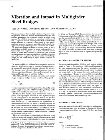
97Wang et al.,. fl.YufiTRAILER912n.13D,y5Ya3YazDty5 l t1(!YuDaytYa1Di,1Dt13K tylFIGURE 1 HS20-44 vehicle model: left, side view; right, front view.Ar roughness coefficient (m3 /cycle)The equations of motion of the bridge are(j)0 discontinuity frequency 1/(271') (cycle/m).(4)The detail of the procedure has been discussed by Wang andHuang (13). In this study, the values of 5 x 10- 6 , 20 x 10- 6 ,80 x 10- 6 , and 256 x 10- 6 m 3/cycle were used according toInternational Organization for Standardization (ISO) specifications (15) as the roughness coefficient Ar for the classesof very good, good, average, and poor roads, respectively.The sample length was taken as 256 m (839.9 ft), and 2,048(2 11 ) data points were generated for this distance. The averagevertical highway surface profiles from five simulations areshown in Figure 2.BRIDGE MODEL AND EQUATIONS OF MOTIONTo study the general impact behavior of steel multigirderbridges, seven highway steel bridges were designed accordingto 1989 AASHTO specifications (1) and the 1982 StandardPlans for Highway Bridges of the U.S. Department of Transportation (16). The span lengths range from 35 to 140 ft(10.67 to 42.67 m). These bridges are designed for the HS2044 loading. Figure 3 (top) shows the typical bridge cross section. All seven bridges consist of five identical girders thatare simply supported. The plan of the bridge with a span of100 ft is given in Figure 3 (bottom); the other bridges havesimilar arrangements. The number of diaphragms for bridgeswith span lengths of 35, 45, 55, 75, 100, 120, and 140 ft (1 ft 0.305 m) are 1, 1, 2, 2, 3, 4, and 5, respectively. Theprimary bridge data are given in Table 1.The multigirder bridges are treated as grillage beam systems(Figure 4). Dynamic response of the bridge was analyzed withfinite element method. The bridge was divided into grillageelements (Figure 5). The node parameters are{8}' { ;}(3)where{8;}{8)wex, 0y [wzi exi eyiF displacement vector of left joint,[wzj exj eyjF displacement vector of right joint,vertical displacement in z-direction, androtational displacements about x- and y-axes, respectively.where[MB] global mass matrix;[KB] global stiffness matrix;[DB] global damping matrix;{8}, {B}, {S} global nodal displacement, velocity, accel-eration vectors; and{FBr} global nodal loading vector, resulting frominteraction between bridge and vehicle.INTERACTION EQUATIONS AND NUMERICALMETHODSThe interaction force of the ith axle between the bridge andvehicle is given as(5)wheretire stiffness of ith axle, tire damping coefficient of ith axle, andU cy; relative displacement between ith axle and bridge Ysi - ( - usri) - ( - Wb;), where Yai verticaldisplacement of ith axle,usri road surface roughness under ith axle (positive upward), andwb; bridge vertical displacement under ith axle (positiveupward); wb; can be evaluated by nodal displacements {8}e of element and displacement interpolation function of element (12); a dot superscript denotes differential with respect to time.The equations of motion of the vehicle are nonlinear, whilethose of the bridge are considered linear. According to thedifferent characteristics of the equations of motion, the fourthorder Runge-Kutta integration scheme (17) was used to solvethe equations of motion of the vehicle, while the solutions ofthose of the bridge were determined by the mode-superposition procedure based on the subspace iteration method. Themain procedure for dynamic analysis of the bridges is discussed elsewhere (12).Kry; Dry;

98TRANSPORTATION RESEARCH RECORD 139321.5 . . - - - - - - - - - - - - - - - - . . . ,lfllfl0.5.sVery Good Road21.5 . . - - - - - - - - - - - - - - - - - - ,Very Good Road.s{/) 0.5lfli:.::ii:.::izz5-0.55-0.5:::;:::;00::-1.5 . .-- -- -- -----'064128192256DISTANCE ALONG THE ROAD (M)2.s2.0 . . - - - - - - - - - - - - - - - - - - ,Good Roadi:.::iz::r:0. 02.s1.0lfl{/)00::-1.5 -- ----- -----'064128192256DISTANCE ALONG THE ROAD (M)lfllfl1----l---\o----l'-t-'---- --.,.-.,.g-i.oi:.::iz::r:2.00::-2.0 . .-- -- -- -----'064128192256DISTANCE ALONG THE ROAD (M)0. 004.0 . . - - - - - - - - - - - - - - - - - - ,Average Road2.s2.0.s{/){/)4.0::r:::r:.g-2.0g-2.000::-4.0 -- ----- -----'064128192256DISTANCE ALONG THE ROAD (M)6.0.------------------,Poor Road02{/){/) --t.ftztll---i-'---v. h-ill\---1'--\f-- i:.::i::r:z::r:00g-3.00.00::-4.0 -- ----- ------'064128192256DISTANCE ALONG THE ROAD (M).s3.0{/){/)0. 0Average Roadlfllfl z --------------,2.0 0.0i:.::il------l.d-----J -.t--n\ff-----'-f' .A- ,-.---10::-2.0 -- ----- -----'064128192256DISTANCE ALONG THE ROAD (M)2·.sGood Road1.0g-1.002 --------------,6.0 . . - - - - - - - - - - - - - - - - - ,3.00 .0 1-- -.J-ll----JH.,.-f'--llo ---- -lg-3.00::-6.0--- -- -- - 064128192256DISTANCE ALONG THE ROAD (M)0::-6.0--- -- -- - 064128. 192256DISTANCE ALONG THE ROAD (M)FIGURE 2 Vertical highway surface profiles: left, right line; right, left line.VIBRATION AND IMPACT CHARACTERISTICSIt is assumed that the bridges have damping characteristicsthat can be modeled as viscous. One percent of critical damping is adopted for the first and second modes according tothe experiment results. The mode-damping coefficients weredetermined by using an approach described by Clough andPenzien (18). To obtain the initial displacements and velocities of vehicle degrees of freedom when the vehicle enteredthe bridge, the vehicle was started in motion at a distance of140 ft (42.67 m, i.e., a five-car length) away from the left endof the bridge and continued moving until the entire vehiclecleared the right end of the bridge. The same class of roadsurface was assumed for both the approach roadways andbridge decks.Table 2 presents the first six frequencies of each bridge.From the table, it is apparent that the first two frequenciesof each bridge-corresponding with bending and torsion modes,respectively-are nearly the same.To learn the space impact characteristics of multigirderbridges, two loading cases, symmetric and asymmetric loadings of a single truck [Figure 6 (top) Loading 1 and Loading2], are considered. Under the conditions of vehicle speed of45 mph (72.41 km/hr) and good road surface, the lateral wheelload distribution factors and impact factors of three bridgeswith span lengths of 35, 55, and 100 ft (10.67, 16.75, and 30.48m), respectively, are computed and shown in Figure 7. Thewheel-load distribution factor acquired for the study is definedas(6)whereFMQt FMQ/nFMQ sum of bending moment or shear of all girders atone section,n number·of wheel-loads in transverse direction, and

213'-6"7'-0"I37'-0"II547'-0"7'-0"II3'-6"'co - C'?25'25'1.I.1.25'25'.1100'Typical analytical bridge: top, typical cross section; bottom, typical plan.FIGURE 3TABLE 1 Properties and Masses of BridgesGirderSpanlengthft***rx 104(in4)r·dx 103(in4)Intermediate diaphragmMass (kips/in)ExteriorgirderInteriorgirder.x 104(in4)Jdx la3(in4)Mass(kips/in)Diaphragm at endsx 104(in4)rJdx 643.9651.9880.0038Inertia moment.Torsional inertia moment.