WIXLIB

3 MethodologyHaving argued in the above section that the Hong Kong listed stock I have is not liquidand hence the key assumption of the heavy traffic model is not satisfied, I start from adescription of order arrivals for different kinds of orders, the dynamics of a limit orderbook is naturally described in the language of queuing theory [2]. Motivated by the factthat it is sufficient to focus on the dynamics of the best bid and ask queue if one isprimarily interested in the level I order book dynamics, I then decided to follow theMarkovian queuing model [2] to test its validity on the data where the limit order book isdriven by orders at the bid and ask side, represented as a system of two interactingMarkovian queues. I will first introduce the setup of R. CONT’s queuing model [2], andthen elaborate my modifications according to the empirical analysis.3.1 ModelSetupTo simplify the initial model, we use the following terms to represent the limit orderbook: The bid price s bt and the ask price sta stb δ , which captures the majority of themarket situation. The size of the bid queue qtb represents the outstanding limit buy orders at the bid.8

The size of the bid queue qta represents the outstanding limit buy orders at the ask.The state of the limit order book is thus described by the triplet X t (stb ,qtb ,qta ) , whichtakes values in the discrete state space δ . 2 .The state X t of the order book is updated by order book events: limit orders (at the bid orask), market orders and cancelations. According to the R.CONT’s works [2], I got theassumption that these events occur according to independent Poisson processes: Market buy (resp. sell) orders arrive at independent, exponential times with rate µ . Limit buy (resp. sell) orders at the (best) bid (resp. ask) arrive at independent,exponential times with rate λ . Cancellations occur at independent, exponential times with rate θ . These events are mutually independent. All orders sizes are equal (assumed to be 1 without loss of generality). All the previous sequences are independent.Under these assumptions qt (qtb ,qta ) is thus a Markov process, taking values in 2 ,whose transitions correspond to the order book events {Ti a ,i 1} {Ti b ,i 1} .9

When the bid or ask orders is depleted, the price moves up or down to the next level ofthe order book. Analogous to the heavy traffic model, the new queue sizes are sampledfrom the empirical PDF f b/a (x, y) . I further assume that the order book contains noempty levels so that these price increments are equal to one tick (in our case, 0.05 HKD): When the bid queue is depleted, the price decreases by one tick. When the ask queue is depleted, the price increases by one tick.In summary, the process X t (stb ,qtb ,qta ) is a continuous-time process withright-continuous, piecewise constant sample paths whose transitions correspond to theorder book events {Ti a ,i 1} {Ti b ,i 1} [2]. At each event: If an order or cancelation arrives on the ask side i.e. T {Ti a ,i 1} :(sTb ,qTb ,qTa ) (sTb ,qTb ,qTa Vi a )1q a V a (sTb δ , Rib , Ria )1q a V aT iT iIf an order or cancelation arrives on the bid side i.e. T {Ti b ,i 1} :(sTb ,qTb ,qTa ) (sTb ,qTb Vi b ,qTa )1qb V b (sTb δ , R'bi , R'ia )1qb V bTiT i(Vi a )i 1 and (Vi b )i 1 are sequences of IID variables, (Ri )i 1 (Rib , Ria )i 1 is a sequence ofIID variables with (joint) distribution f b (x, y) , and ( R'i )i 1 ( R'bi , R'ia )i 1 is a sequence ofIID variables with (joint) distribution f a (x, y) .10

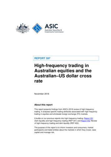
3.2ModelModifications3.2.1 EventArrivalRateIn R. CONT’s original model [2], all kinds of orders arrive at an exponential rate, which Idoubt maybe is not the case in our data, so I run some empirical study about the orderarrival rate. I first differentiated 6 different kinds of orders from our data, which is: LimitBuy Orders, Limit Sell Orders, Market Buy Orders, Market Sell Orders, CancellationBuy Orders, and Cancellation Sell Orders. In our terms, Limit Buy means someoneposted a buy order at the best bid, and Limit Sell means someone posted a sell order atbest ask. Market Buy means someone takes the best bid offers, and Market Sell meanssomeone takes the best ask offers. Cancellation Buy means someone cancelled their bidorders at the best bid, and Cancellation Sell means someone cancelled their ask orders atthe best ask. Fig 1 shows the empirical probability distribution of the six different kindorders arrival rate:11

Limit Buy OrdersLimit Sell 20406080Market Buy Orders100120140160180200Market Sell 00350400450002040Cancellation Buy Orders6080100120140160Cancellation Sell 040050060000100200300400500600Fig 1. Order arrival distribution and the exponential distribution.In Fig 1, the white line indicates the best fitted exponential distribution. It is observedthat, in some cases, the exponential distribution fits the data well, such as limit buy ordersand market sell orders, but in some other cases, such as cancellation buy orders andmarket buy orders, the exponential distribution obviously fails to fit the data.This empirical study suggests that one potential threat of R. CONT’s Queuing Model [2]might be the exponential arrival rate, so I try to figure out another distribution that maycapture the arrival rate better than exponential, and I found one candidate after some trialand error, which is called Weibull Distribution, which is often used to describe the size12

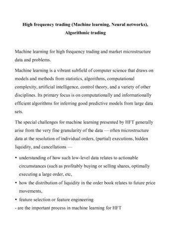
distribution of particles. The probability density function of a Weibull random variable xkis f (x; λ ,k) k / λ (x / λ ) k 1 e ( x/ λ ) 1(x 0)I then try to fit the arrival rate using the Weibull distribution. The results are shown in Fig2:Limit Buy OrdersLimit Sell 20406080Market Buy Orders100120140160180200Market Sell 00350400450002040Cancellation Buy Orders6080100120140160Cancellation Sell 040050060000100200300400500600Fig 2. Order arrival distribution and the Weibull distribution.In Fig 2, the white line indicates the exponential distribution and the red one is theWeibull distribution. To access the goodness of fitting, I also look at the Q-Q plots asshown in Fig 3.13

Fig 3. Q-Q plots of the real data against the Weibull distribution or the exponentialdistribution.In Fig 3, it shows the comparison between the Weibull distribution and the exponentialdistribution in each order figure. The blue lines indicate the authentic data, while the redlines are the calculated distribution. The closeness indicates the accuracy of thedistribution to the real data. One can then clearly see that nearly for each figure, theWeibull distribution outperforms Exponential, especially for Limit Sell Orders, MarketBuy Orders, Cancellation Buy Orders and Cancellation Sell Orders, where we say thatthe Weibull distribution is really a good fit to the data. After these empirical studies, I14

decided to use the Weibull distribution instead of the exponential distribution tocharacterize the arrival rate of different orders.3.2.2 OrderSizeAnother concern I have about the original model is the assumption that all coming ordershave unit lot size (400 shares), which I believe is quite biased from the reality. I first runa study to analyze the order size distribution, as is shown in Fig 4.Limit Buy OrdersLimit Sell 050006000700080009000 1000000100020003000Market Buy Orders400050006000700080009000 10000700080009000 10000700080009000 10000Market Sell 050006000700080009000 1000000100020003000Cancellation Buy Orders400050006000Cancellation Sell 50006000700080009000 1000000100020003000400050006000Fig 4. Order size distribution.15

It’s obvious to see that the order size follows an exponential distribution as well, which Ibelieve is close to the reality, so I decided to add order size as another random variable toform a compound renewal process, in which we use the Weibull distribution again tocharacterize its dynamics.3.2.3 EventCorrelationThe last doubt I have is that I believe all the events should have some inner connectionbetween each other, whereas the original model claims that orders are independent. I firstcalculated the correlation between all kind of orders arrival duration and its related size inChart 1.Chart 1. Order duration and size correlation matrix.16

The above 12 12 correlation matrix is distributed as following: Limit Buy OrdersDuration at the first row, Limit Buy Orders Size at the second row, Limit Sell OrdersDuration at the third row, Limit Sell Orders Size at the forth row, and so on. Thehighlighted items are those with high correlation, and I pick them up in Chart 2.Chart 2. High correlation entries.One thing I found really interesting is the correlation between limit buy duration andmarket sell duration. The high correlation could be explained by the basic economicprinciples, where limit buy orders represented demand. The high demand will boost theprice, according to the economic principles, so people will tend to buy more shares togain profit, and that’s why market sell orders appears so soon. Another interesting fact isthat the size correlation is relatively small, so we could say that the size is an independentfactor in the queuing system. So I integrated the correlation of limit buy duration and17

market sell duration using the same empirical distribution function f (x, y) , as isdescribes in the previous session.3.3 ModelApplicationAfter having the Markovian queuing model discussed above, I hypothesized that themodel could accurately simulation the dynamics of the real market. Having thishypothesis in mind, I start to test multiple trading strategies based on this model,especially for market makers.3.3.1 MarketMakingIn practice, it is of great interest to understand the mechanism of basic market makingactivities and the impact of possible strategies. Intuitively, market makers reap profits byposting same size ask and bid order simultaneously, selling highly and buying low. Here,I consider the following model problem. Suppose the market maker posts N shares attime t, and he is obliged to close his position with completion time T, that is, close Nshare position in [t,t T ] . The market maker could post limit order on any level of orderbook he want, and he is expecting other traders in the market could hit both his bid orderand ask order. The market maker must close his position at time t T by purchasing(selling) the remaining position at market price. The most important decision the marketmaker has to make is which level he should put the order at. It’s conceptual obvious thatposting orders at a deeper position (closer to market price) will increase the execution18

probability while acquiring small profit, and posting orders further will get more profit bytaking more risk. In reality, most market maker will have a targeting profit margin andrisk tolerance threshold. Then it is not obvious quantify the results of putting orders ondifferent levels. I tested this market making strategies with different completion time T,number of shares N and level of order placement by running independent Monte Carlosimulation. The results will be analyzed in the Discussion session.3.3.2MarketMakingwithbalancingstrategyThe previous study on the market making activities is the simplest version. Here, weconsidered a more complex situation. Normally, rather than leaving the portfolio aloneafter posting the initial shares at time t (which is the assumption in the previous strategy),most market makers will follow the trend of the market and modify the portfolioaccording to the market performance in real time. One normal strategy is to rebalance theposition around the current price, since it assures the equal probability for both sides to beexecuted. Here, besides the model problems in the previous session, I also integrated thebalancing strategy, which shows as follows:At each end of time interval Δt If currently no position is on the best level and both bid and ask size hasn’t beendepleted yet, rearrange the remaining shares to be balanced around the currentmarket price.19

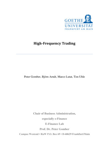
If both sides haven’t been depleted and the current price is already balanced,decrease the margin of both sides by one tick. If one size already depleted, try to increase the other side by one tick.In the model setup, I ignore the cancellation fee for cancellation the original orders, sincein most exchanges, there will be a “liquidity award” for posting limit order, which isapproximately the same amount of the cancellation fee. I tested this balancing strategiesagain with different completion time T, number of shares N and level of order placementby running independent Monte Carlo simulation. The results will be analyzed in the nextsession.3.3.3 SmokingStrategyIt is highly interesting to understand the high frequency market maker’s trick beyond thebasic market making strategy. One of the widely used strategies is called SmokingStrategy. High-Frequency traders place small alluring quotes to attract other side’smarket order. Suppose another party detects this alluring quote (usually throughautomated trading system), they will then send out a market order. Since market ordersare only executed at the best market price, HF traders can cancel the quotes before themarket orders arrive, thus letting the other party hits the large shares previous posted byHF traders. Fig 5 illustrated one example of the smoking strategy.20

Fig 5. An example of smoking strategy.The smoking strategy could be happened in both ask and bid side. The key for thesmoking strategy is the speed, which is exactly the advantage of high-frequency traders. Iexamined the 5 days Hong Kong traded stock data I have, and found out that there are 20occurrences happened in 5 days (7 bid side, 13 ask side). The average alluring quote sizeis 7,280 shares, the average cancellation duration is 1.98s, and the average tradingvolume is 2,160 shares. The histogram of cancellation duration is shown in Fig 6.21

14121086420012345678910Fig 6. Cancellation duration histogram.Understood that the prime parameter for the success of smoking strategy is thecancellation duration, I tested the smoking strategy based on the model by runningindependent Monte Carlo simulation. The result will be discussed in the next session.22

4 Discussion4.1 ModelSimulationResultsTo sum up the methodology, I employed a Markovian Queuing Model [2] whosetransition corresponds to the order book events {Ti a ,i 1} {Ti b ,i 1} . There are six kindsof orders in the system. For limit buy orders and market sell orders, I use the empiricalprobability distribution to generate the simulation queue. Other than that, thecorresponded Weibull distribution is used. The order size and duration are seen asindependent to each other. The final simulation queue contains around 12,000 events in aday. The details are documented in Chart 3.Chart 3. Discrete event simulation statistics.23

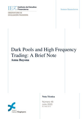
Based on this queue, I ran a simple simulation to test the validity of this model. Thesimulation starts with the first price of the first day, and one sample path is shown in Fig7 where the red line is the real first day data, and the blue line is the simulated result. Onecan tell that the simulation results catch the sense of our market pretty 012000140001600018000Fig 7. A sample path of simulated stock prices.4.2 MarketMakingSimulationResultsAccording to the previous discussion, I tested the market making strategy based on theMarkovian Queuing System. The parameter is nLevel, which range from 0 to 5,24

representing the level market maker put the orders; Completion Time T, which rangefrom 3600s to 18000s (1 to 5 hours), representing the total amount of time for closing theposition; Number of shares N, which range from 400 to 2,000, representing the totalshares used by the market making strategy. The results are shown in the followingfigures:Comple

dynamic of HFT market, to HFT data, which recorded the Limit Order Book of a HK-traded stock for one week. I assume that the model could accurately simulate the real market behavior, upon which I apply and test different trading strategies. The final deliverable includes a market simulation model