WIXLIB

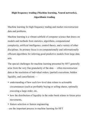
High frequency trading (Machine learning, Neural networks),Algorithmic tradingMachine learning for high frequency trading and market microstructuredata and problems.Machine learning is a vibrant subfield of computer science that draws onmodels and methods from statistics, algorithms, computationalcomplexity, artificial intelligence, control theory, and a variety of otherdisciplines. Its primary focus is on computationally and informationallyefficient algorithms for inferring good predictive models from large datasets.The special challenges for machine learning presented by HFT generallyarise from the very fine granularity of the data — often microstructuredata at the resolution of individual orders, (partial) executions, hiddenliquidity, and cancellations — understanding of how such low-level data relates to actionablecircumstances (such as profitably buying or selling shares, optimallyexecuting a large order, etc, how the distribution of liquidity in the order book relates to future pricemovements, feature selection or feature engineering- are the important process in machine learning for HFT

High Frequency Data for Machine LearningHigh frequency trading - holding periods, order types (e.g. passive versusaggressive), and strategies (momentum or reversion, directional orliquidity provision, etc.).Data driving HFT activity tends to be the most granular available.Typically microstructure data - every order placed, every execution, andevery cancellation, and reconstruction (at least for equities) of the fulllimit order book.A single day’s worth of microstructure data on a highly liquid stock ismeasured in gigabytes. Storing this data historically for any meaningfulperiod and number of names requires both compression and significantdisk usage; processing this data efficiently generally requires streamingthrough the data by only uncompressing small amounts at a time.What systematic signal or information is contained in microstructuredata? - What “features” or variables can we extract from this extremelygranular, lower-level data.

Limit Order Trading and Market SimulationLimit order markets: By this we mean that buyers and sellers specifynot only their desired volumes, but their desired prices as well. A limitorder to buy (respectively, sell) V shares at price p may partially orcompletely execute at prices at or below p (at or above p).For example, suppose that NVIDIA Corp. (NVDA) is currently trading atroughly 27.22 a share (see Figure 1, which shows an actual snapshot ofan NVDA order book), but we are only willing to buy 1000 shares at 27.13 a share or lower. We can choose to submit a limit order with thisspecification, and our order will be placed in the buy order book, which isordered by price, with the highest price at the top (this price is referred toas the bid; the lowest sell price is called the ask). In the exampleprovided, our order would be placed immediately after the extant orderfor 109 shares at 27.13; though we offer the same price, this order hasarrived before ours. If an arriving limit order can be immediatelyexecuted with orders on the opposing book, the executions occur. Forexample, a limit order to buy 2500 shares at 27.27will cause executionwith the limit sell orders for 713 shares at 27.22, and the 1000-share and640-share sell orders at 27.27, for a total of 2353 shares executed. Theremaining (unexecuted) 147 shares of the arriving buy order will becomethe new bid at 27.27. It is important to note that the prices of executionsare the prices specified in the limit orders already in the books, not theprices of the incoming order that is immediately executed. Thus wereceive successively worse prices as we consume orders deeper in theopposing book.

Performance and policies found by RL vary with stock properties such asliquidity, volume traded, and volatilitySubmit and leave (S&L) policiesState-based strategies – strategies that can examine salient features of thecurrent order books and our own activity – in order to decide what to donext.Variables: elapsed time t, remaining inventory i, which represent howmuch time of the horizon H has passed and how many shares we haveleft to execute in the target volume V. Different resolutions of accuracywill be investigated for these variables, which we refer to as privatevariables, since they are essentially only known and of primary concernto our execution strategy. More precisely, we pick I and T, which are the

resolutions (maximum values) of the private variables i and t,respectively. I represents the number of inventory units our policy candistinguish between – if V 10,000 shares, and I 4, our remaininginventory is represented in rounded units of V/I 2,500 shares each.Similarly, we divide the time horizon H into T distinct points at whichthe policy is allowed to observe the state and take an action; for H 2 minand T 4 we can submit a revised limit order every 30 seconds, and thetime remaining variable t can assume values from 0 (start of the episode)down to 4 (last decision point of the episode).Additional state variables: market variables, a state has the formxm t, i, o1, , oR , where the oj are market variables.Action space: simple limit order price at which to reposition all of ourremaining inventory, for the problem of selling V shares, action acorresponds to placing a limit order for all of our unexecuted shares atprice ask - a. Thus we are effectively withdrawing any previousoutstanding limit order we may have (which is indeed supported by theactual exchanges), and replacing with a new limit order. Thus a may bepositive or negative, with a 0 corresponding to coming in at the currentask, positive a corresponding to "crossing the spread" towards the buyers,and negative a corresponding to placing our order in the sell book.Rewards: An action from a given state may produce immediate rewards,which are essentially the proceeds (cash inflows or outflows, dependingon whether we are selling or buying) from any (partial) execution of thelimit order placed. Furthermore, since we view the execution of all V

shares as mandatory, any inventory remaining at the end of time Hisimmediately executed at market prices --- that is, we eat into theopposing book to execute, no matter how poor the prices, since we haverun out of time and have no choice.Measure the execution prices achieved by a policy relative to the midspread price (ask bid)/2 at the start of the episode in question. Thus, weare effectively comparing performance to the idealized policy which canexecute all V of its shares immediately at the mid-spread, and thus areassuming infinite liquidity at that point.Trading cost of a policy: the underperformance compared to themidspread baseline.We assume that commissions and exchange fees are negligible.

Predicting Price Movement from Order Book StateLearn models that themselves profitably decide when to trade and how totrade: The development of features that permit the reliable prediction ofdirectional price movements from certain states. By “reliable” we donot mean high accuracy, but just enough that our profitable tradesoutweigh our unprofitable ones. The development of learning algorithms for execution that capture thispredictability or alpha at sufficiently low trading costs.First find profitable predictive signals: Bid-Ask Spread: Price: A feature measuring the recent directional movement ofexecuted prices. Smart Price: A variation on mid-price where the average of the bid andask prices is weighted according to their inverse volume. Trade Sign: A feature measuring whether buyers or sellers crossed thespread more frequently in recent executions. Bid-Ask Volume Imbalance: Signed Transaction Volume:Features above were normalized. In order to obtain a finite state space,features were discretized into bins in multiples of standard deviationunits.

Learning algorithm: buying 1 share at the bid-ask midpoint and holdingthe position for t seconds, at which point we sell the position, again at themidpoint; and the opposite action, where we sell at the midpoint and buyt seconds later. In the first set of experiments we describe, we considereda short period of t 10 seconds.The methodology can now be summarized as follows:For each of 19 names, order book reconstruction on historical data wasperformed.At each trading opportunity, the current state (the value of the sixmicrostructure features described above) was computed, and the profit orloss of both actions (buy then sell, sell then buy) is tabulated via orderbook simulation to compute the midpoint movement.Learning was performed for each name using all of 2008 as the trainingdata. For each state 𝑥 in the state space, the cumulative payoff for bothactions across all visits to 𝑥 in the training period was computed.Learning then resulted in a policy π mapping states to action, where 𝜋(𝑥)is defined to be whichever action yielded the greatest training setprofitability in state 𝑥.Testing of the learned policy for each each name was performed usingall 2009 data. For each test set visit to state 𝑥, we take the action 𝜋(𝑥)prescribed by the learned policy, and compute the overall 2009profitability of this policy.

FIGURE 4: Correlations between feature values and learned policies. Foreach of the six features and 19 policies, we project the policy onto justthe single feature compute the correlation between the feature value andaction learned ( 1 for buying, -1 for selling). Features indices are in theorder Bid-Ask Spread, Price, Smart Price, Trade Sign, Bid-Ask VolumeImbalance, Signed Transaction Volume.

FIGURE 5: Comparison of test set profitability across 19 names forlearning with all six features (red bars, identical in each subplot) versuslearning with only a single feature (blue bars).

Optimal strategy found: momentum behaviour for time periods of milliseconds to seconds, reversion strategies for dozens of seconds to several minutesAspects that one must consider when applying machine learning to highfrequency data: the nature of the underlying price formation process, andthe role and limitations of the learning algorithm itself.

Empirical Limitations on High Frequency Trading ProfitabilityEmpirical study estimating the maximum possible profitability of themost aggressive such practices: trading strategy exclusively employingmarket orders and relatively short holding periods.The overarching fear is that quantitative trading groups, armed withadvanced networking and computing technology and expertise, are insome way victimizing retail traders and other less sophisticated parties.The HFT debate often conflates distinct phenomena, confusing, forinstance, dark pools and flash trading, which are essentially new marketmechanisms, with HFT itself, which is a type of trading behaviourapplicable to both existing and emerging exchanges. The core concernregarding HFT, however, is relatively straightforward: that the ability toelectronically execute trades on extraordinarily short time scales,combined with the quantitative modelling of massive stores of historicaldata, permits a variety of practices unavailable to most parties. A broadexample would be the discovery of very short-term informationaladvantages (for instance, by detecting large, slow trades in the market)and profiting from them by trading rapidly and aggressively.We demonstrate an upper bound of 21 billion for the entire universe ofU.S. equities in 2008 at the longest holding periods, down to 21 millionor less for the shortest holding periods (see discussion of holding periodsbelow). Furthermore, we believe these numbers to be vast overestimatesof the profits that could actually be achieved in the real world. Thesefigures should be contrasted with the approximately 50 trillion annual