WIXLIB

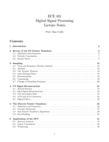
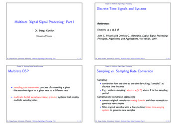
Chapter 9Basic Signal ProcessingMotivationMany aspects of computer graphics and computer imagery differ from aspects ofconventional graphics and imagery because computer representations are digital anddiscrete, whereas natural representations are continuous. In a previous lecture wediscussed the implications of quantizing continuous or high precision intensity values to discrete or lower precision values. In this sequence of lectures we discuss theimplications of sampling a continuous image at a discrete set of locations (usuallya regular lattice). The implications of the sampling process are quite subtle, and tounderstand them fully requires a basic understanding of signal processing. Thesenotes are meant to serve as a concise summary of signal processing for computergraphics.ReconstructionRecall that a framebuffer holds a 2D array of numbers representing intensities. Thedisplay creates a continuous light image from these discrete digital values. We saythat the discrete image is reconstructed to form a continuous image.Although it is often convenient to think of each 2D pixel as a little square thatabuts its neighbors to fill the image plane, this view of reconstruction is not verygeneral. Instead it is better to think of each pixel as a point sample. Imagine animage as a surface whose height at a point is equal to the intensity of the image atthat point. A single sample is then a “spike;” the spike is located at the position ofthe sample and its height is equal to the intensity associated with that sample. Thediscrete image is a set of spikes, and the continuous image is a smooth surface fittingthe spikes as shown in Figure 9.1. One obvious method of forming the continuoussurface is to interpolate between the samples.1

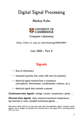
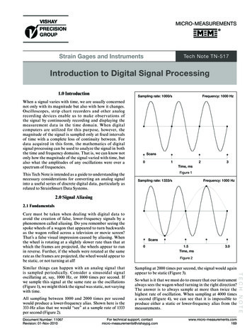
2CHAPTER 9. BASIC SIGNAL PROCESSINGFigure 9.1: A continuous image reconstructed from a discrete image represented asa set of samples. In this figure, the image is drawn as a surface whose height is equalto the intensity.SamplingWe can make a digital image from an analog image by taking samples. Most simply,each sample records the value of the image intensity at a point.Consider a CCD camera. A CCD camera records image values by turning lightenergy into electrical energy. The light sensitive area consist of an array of smallcells; each cell produces a single value, and hence, samples the image. Notice thateach sample is the result of all the light falling on a single cell, and corresponds toan integral of all the light within a small solid angle (see Figure 9.2). Your eye issimilar, each sample results from the action of a single photoreceptor. However, justlike CCD cells, photoreceptor cells are packed together in your retina and integrateover a small area. Although it may seem like the fact that an individual cell of aCCD camera, or of your retina, samples over an area is less than ideal, the fact thatintensities are averaged in this way will turn out to be an important feature of thesampling process.A vidicon camera samples an image in slightly different way than your eye ora CCD camera. Recall that television signal is produced by a raster scan process inwhich the beams moves continuously from left to right, but discretely from top tobottom. Therefore, in television, the image is continuous in the horizontal direction.and sampled in the vertical direction.The above discussion of reconstruction and sampling leads to an interesting question: Is it possible to sample an image and then reconstruct it without any distortion?Jaggies, AliasingSimilarly, we can create digital images directly from geometric representations suchas lines and polygons. For example, we can convert a polygon to samples by testing

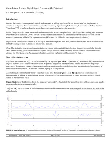
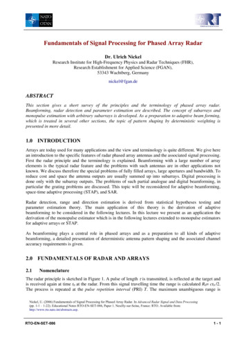
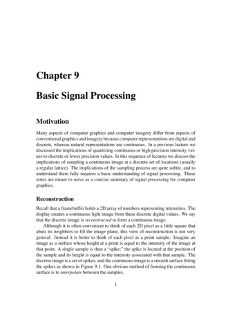
3Figure 9.2: A CCD camera. Each cell of the CCD array receives light from a smallsolid angle of the field of view of the camera. Thus, when a sample is taken the lightis averaged over a small area.whether a point is inside the polygon. Other rendering methods also involve sampling: for example, in ray tracing, samples are generated by casting light rays intothe 3D scene.However, the sampling process is not perfect. The most obvious problem is illustrated when a polygon or checkerboard is sampled and displayed as shown in Figure 9.3. Notice that the edge of a polygon is not perfectly straight, but instead isapproximated by a staircased pattern of pixels. The resulting image has jaggies.Another interesting experiment is to sample a zone plate as shown in Figure 9.4.Zone plates are commonly used in optics. They consist of a series of concentricrings; as the rings move outward radially from their center, they become thinner andmore closely spaced. Mathematically, we can describe the ideal image of a zone . If we sample the zone plateplate by the simple formula: (to sample an image given by a formula at a point is very easy; we simplyplug in the coordinates of the point into the function ), rather than see a single setof concentric rings, we see several superimposed sets of rings. These superimposedsets of rings beat against one another to form a striking Moire pattern.These examples lead to some more questions: What causes annoying artifactssuch as jaggies and moire patterns? How can they be prevented?Digital Signal ProcessingThe theory of signal processing answers the questions posed above. In particular, itdescribes how to sample and reconstruct images in the best possible ways and howto avoid artifacts dues to sampling.

4CHAPTER 9. BASIC SIGNAL PROCESSINGFigure 9.3: A ray traced image of a 3D scene. The image is shown at full resolutionon the left and magnified on the right. Note the jagged edges along the edges of thecheckered pattern.Signal processing is very useful tool in computer graphics and image processing.There are many other applications of signal processing ideas, for example:1. Images can be filtered to improve their appearance. Sometimes an image hasbeen blurred while it was acquired (for example, if the camera was moving)and it can be sharpened to look less blurry.2. Multiple signals (or images) can be cleverly combined into a single signal,so that the different components can later be extracted from the single signal.This is important in television, where different color images are combined toform a single signal which is broadcast.Frequency Domain vs. Spatial DomainThe key to understanding signal processing is to learn to think in the frequency domain.Let’s begin with a mathematical fact: Any periodic function (except various monstrosities that will not concern us) can always be written as a sum of sine and cosinewaves.

5Figure 9.4: Sampling the equation . Rather than a single set of ringscentered at the origin, notice there are several sets of superimposed rings beatingagainst each other to form a pronounced Moire pattern.

CHAPTER 9. BASIC SIGNAL PROCESSING6A periodic function is a function defined in an interval that repeats itself outside the interval. The sine function— ! —is perhaps the simplest periodic function and has an interval equal to " # . It is easy to see that the sine function is periodicsince % " # &' ( . Sines can have other frequencies, for example, the sinefunction ")# repeats itself times in the interval from * to " # . is the frequency of the sine function and is measured in cycles per second or Hertz.If we could represent a periodic function with a sum of sine waves each of whoseperiods were harmonics of the period of the original function, then the resulting sumwill also be periodic (since all the sines are periodic). The above mathematical factsays that such a sum can always be found. The reason we can represent all periodicfunctions is that we are free to choose the coefficients of each sine of a differentfrequency, and that we can use an infinite number of higher and higher frequencysine waves.As an example, consider a rather nasty function—a square pulse. This function isnasty because it is discontinuous in value and derivative at the beginning and endingpoints of the pulse. A square pulse is the limit as -, . of0/ 0 1 2 34"5 #" "4687:9"48;# 6 9) ")?")?;;4 A@& 4F @& G E4H B C@& D;EF 4 H @I J LK K KM Where the angular frequency (in radians) @L ")# . A plot of this formula for fourdifferent values of is shown in Figure 9.5. Notice that as increases, the sum ofsines more closely approximates the ideal square pulse.More generally, a non-periodic function can also be represented as a sum of sin’sand cos’s, but now we must use all frequencies, not just multiples of the period. Thismeans the sum is replaced by an integral.1 N O 4PRQ QTS" #U@V XW Y[Z]\ ]@ f@V @& % bac @& ( aIed ;where W Y Z \are the coefficients of each sine4 . Sf@V is called the spectrum of the function 1 2 .and cosine; SThe spectrum can be computed from a signal using the Fourier transform.SU@V OPRQ Q 1 N XW Y Z \ c Unfortunately, we do not have time to derive these formulas; the reader will have toaccept them as true. For those interested in their derivation, we refer you to Bracewell.

7///9 / 9hgFigure 9.5: Four approximations to a square pulse. Notice that each approximationinvolves higher frequency terms and the resulting sum more closely approximatesthe pulse. As more and more high frequencies are added, the sum converges exactlyto the square pulse. Note also the oscillation at the edge of the pulse; this is oftenreferred to as the Gibbs phenomena.

CHAPTER 9. BASIC SIGNAL PROCESSING8To illustrate the mathematics of the Fourier transform, let us calculate the Fouriertransform of a square pulse. A square pulse is described mathematically as8icj k]lXmc 2 Oonp*9 4p prq 9prs The Fourier transform of this function is straightforward to compute.PGQ QXiCjtk]l8mr 2 W Pwx vY Z \u c W vx W Y[Z]\;(aU@W Y xv Z 9 @ Y Z \y c xv p vx;zW9a @" 9@ Y xv Z Here we introduce the function defined to be { ## Note that # equals zero for all integer values of , except equals zero. At zero,the situation is more complicated: both the numerator and the denominator are zero.However, careful analysis shows that *4 .Thus, Oon*4 * w *A plot of the sinc function is shown below. Notice that the amplitude of the oscillation decreases as moves from the origin.

9It is important to build up your intuition about functions and their spectra. Figure 9.6 shows some example functions and their Fourier transforms.The Fourier transform of !@& is two spikes, one at ;V@ and the other at V@ .This should be intuitively true because the Fourier transform of a function is an expansion of the function in terms of sines and cosines. But, expanding either a singlesine or a single cosine in terms of sines and cosines yields the original sine or cosine.Note, however, that the Fourier transform of a cosine is two positive spikes, whereasFourier transform of a sine is one negative and one positive spike. This follows fromthe property that the cosine is an even function ( 2;V@O} B C@O} ) whereas the sineis an odd function ( ; @O}Oe; @O} ).The Fourier transform of a constant function is a single spike at the origin. Onceagain this should be intuitively true. A constant function does not vary in time orspace, and hence, does not contain sines or cosines with non-zero frequencies.Comparing the formula for the Fourier transform with the formula for the inverseFourier transform, we see that they differ only in the sign of the argument to theexponential. This implies that Fourier transform and the inverse Fourier transformare qualitatively the same. Thus, if we know the transform from the space domainto the frequency domain, we also know the transform from the frequency domain tothe space domain. Thus, the Fourier transform of a single spike at the origin consistsof sines and cosines of all frequencies equally weighted.In the above discussion we have used the term spike several times without properly defining it. A delta function has the property that it is zero everywhere except at the origin. 2 * *The value of the delta function is not really defined, but its integral is. That is,PRQ 2 c 4