Transcription
Methods of long chain branching detection in PE by triple-detector gelpermeation chromatographyThipphaya Pathaweeisariyakul,1 Kanyanut Narkchamnan,1 Boonyakeat Thitisuk,1 Wallace Yau21Siam Cement Group (SCG), SCG Chemicals Co., Ltd., 10 I-1 Road, Map Ta Phut Industrial Estate, Muang District, RayongProvince 21150, Thailand2Polymer Characterization Consultant, USA, www.linkedin.com/pub/wallace-yauCorrespondence to: T. Pathaweeisariyakul (E - mail: thipphap@scg.co.th)Long chain branching (LCB) in polyethylene is one of the key microstructures that controls processing and final properties. Gel permeation chromatography (GPC) with viscometer (IV) and/or light scattering (LS) has been intensely used to quantifyLCB. The widespread method to quantify LCB from GPC with IV or LS is the method of LCB frequency (LCBf) based on theZimm–Stockmayer (ZS) random branching model. In this work, the conventional approach was compared with the recently developed method, called gpcBR. The comparison of the sensitivity of both methods is made on highly branched polymer, that is, variousgrades of commercial LDPE and also on polymer with very low level of LCB, that is, a commercial HDPE with no LCB, convertedinto several branched test samples of gradually increasing LCB by multiple extrusion. Finally, the linkages of LCB quantities fromboth methods to the rheological data and processing properties are illustrated. The new gpcBR index can access lower LCB level andshows obviously better relationship with both rheological data and processing properties than LCBf from the conventional ZS model.ABSTRACT:C 2015 Wiley Periodicals, Inc. J. Appl. Polym. Sci. 2015, 132, 42222.VKEYWORDS: polyolefins; properties and characterization; structure-property relationsReceived 12 December 2014; accepted 10 March 2015DOI: 10.1002/app.42222INTRODUCTIONIn polyethylene technology, long chain branching (LCB) is animportant microstructure to control many processing properties, such as melt viscosity, melt strength, die swell ratio, and soforth.1,2 For example, in LDPE extrusion coating process, LCBstructure can improve neck-in properties.3,4 In pipe technology,high LCB level will change some important properties, such asslow crack growth.5 Researchers thus attempted to control LCBlevel occurred in manufacturing process. To support the polymer design development, a well-defined characterization technique for LCB is required. A widespread tool to achieve thisapproach is gel permeation chromatography (GPC) with hightemperature capability, connected with viscosity detector (IV),or light scattering (LS) detector, or both (3D-GPC).6–10The quantification of LCB of polymer by GPC with triple detectors is commonly based on a LCB frequency (LCBf) calculationwith the assumption of the Zimm–Stockmayer (ZS) randombranching model.6,10,11 In this article from this point on, wewill refer this approach as the “current or conventional 3D-GPCmethod of determining LCB.” With the same molecular weight,the root-mean-square radius (Rg) of a branch polymer issmaller than that of a linear polymer. The branching index (g)factor is defined as the ratio of the Rg square of the branchedpolymer over that of a linear polymer of same molecularweight, as shown in eq. (1). Similarly, the branching index fromintrinsic viscosity (g’) can also be defined as the ratio of intrinsic viscosity ([g]) of a branch polymer over the [g] of linearpolymer of same molecular weight, as shown in eq. (2). Thesetwo indices are related with an exponent power E, so calledstructure factor, as shown in eq. (3).g5 Rg 2 branch Rg 2 linear g’5½g branch g linearg’ 5ge(1)(2)(3)To estimate g (Rg) from g’ ([g]), a value of this epsilon (e)parameter must be assumed. The problem is that, this structurefactor can vary from 0.5 to 1.5, depending on molecular architecture9 and recently it was found to be depending on degree ofpolymerization.12 It is even more challenging for LDPE whichhas very complex branching architectures.From g or g’ value, the average LCB per molecule (B) can beestimated from the ZS equation (eq. (4)).C 2015 Wiley Periodicals, Inc.VWWW.MATERIALSVIEWS.COM42222 (1 of 9)J. APPL. POLYM. SCI. 2015, DOI: 10.1002/APP.42222
ARTICLEWILEYONLINELIBRARY.COM/APP! ! 6 1 21B 1 2ð21B Þ1 2 1B 1 2g5ln21B 2Bð21B Þ1 2 2B 1 2(4)From the B value obtained from eq. (4), LCBf, a number ofLCB per 1000 carbon can be calculated by using eq. (5).10005number of LCB per 1000 carbon (5)LCBf 5k5R B MWhere, M is molecular weight, and R is a factor of the repeatingmolecular weight unit. For example, polyethylene, R 5 (14 114)/2 5 14, or for PVC, R 5 (14 1 13 1 35)/2 5 31.A new branching approach, gpcBR, has been recently introduced to analyze LCB by 3D-GPC by Yau and co-workers.13,14Comparing to the traditional g or g’ and LCBf parameter, thisnew gpcBR index provides a measure of polymer branchinglevel with a much improved precision, by combining intrinsicviscosity and absolute MW measurements from viscometer (IV)and LS detectors. The expression of gpcBR isgpcBR5 KM aV ;CC½g CCMW aMW a 21 521½g MW ;CC½g MW ;CC(6)Where MW,CC and [g]CC are the molecular weight and intrinsicviscosity from conventional GPC calculation assuming polymeris linear with no LCB. The [g] term is the actual intrinsic viscosity, which is the measured value from the online IV, calculated by the IV peak area method for high precision. MW is theweight average of absolute molecular weight from LS detector,also calculated by the LS peak area method for high precision.The interpretation of gpcBR is simple and straight forward. Forlinear polymers, gpcBR will be close to zero. For branched polymers, gpcBR will be higher than zero. In fact, gpcBR value represents the fractional [g] change due to the molecular sizecontraction effect as the result of polymer branching. A gpcBRvalue of 0.5 or 2.0 would mean a molecular size contractioneffect of [g] at the level of 50 and 200%, respectively.The ratio of [g]CC/[g] or MW/MW,CC have been used in the literature for measuring polymer LCB, but neither of them byitself can provide good enough precision for practical application. This is because the terms [g]CC and MW,CC in the ratioexpressions are subjected to variations in experimental conditions of instrument band broadening, elution curve baselinecutting, and variations on the conventional GPC calibrationcurve itself. This problem of variation in [g]CC and MW,CC ishowever nicely compensated for in the gpcBR formulation (seethe right side of eq. (6)), because these two terms appeartogether in the gpcBR formulation but in the opposite way tocancel out the errors, that is, [g]CC being in the numerator andMW,CC being in the denominator. This is the reason to givegpcBR the characteristic of much higher precision than eitherthe [g] or MW ratio. The presence of the ratio of MV,CC/MW,CCin the gpcBR formulation (see the middle portion of eq. (6)) isalso helpful in compensating for the molecular weight polydispersity differences among industrial samples. That too helps toprovide gpcBR with good precision characteristics.WWW.MATERIALSVIEWS.COMIn this work, the conventional method of LCBf based on ZSmodel and gpcBR derived from same 3D-GPC data were compared based on the following systems, linear polyethylene,highly branched polyethylene, and polyethylene with very lowlevel of LCB. In addition, both LCB indices from 3D-GPC wererelated to a simple LCB index from rheological technique andlastly linked to polymer processing property.EXPERIMENTALFirst of all, a linear sample, SRF1475a (Polyethylene standard)(NIST, USA) was selected to confirm the measurement reliability and create the linear baseline of the LCBf and gpcBR value.For branched polymer, we selected a commercial LDPE as ahighly branched polymer (LD-1), and a commercial HDPE withno LCB (HD-1), which is transformed into several branchedtest samples of gradually increasing LCB by multiple extrusion.LDPE sample was measured 10 times on a high temperatureGPC instrument with triple detectors (Polymer Char, Spain):they are IR5 detector, IV, and an 8-angle LS detector (WyattTechnology, assembled by Polymer Char). The dual IR wavelength capability of the IR5 detector allows the short chainbranching (SCB) distribution to be measured across the GPCelution curve. The equipment including control and analysissoftware was from Polymer Char. This SRF1475a sample wasinitially used to investigate the sensitivity and precision of thefollowing methods: first is the current LCBf method based onZS branching model, and second is the recently developedgpcBR method. The second model sample is a linear HDPE,which is passed several times through the twin screw extruderat 200oC, Haake, Germany, to generate LCB from thermal/sheardegradation. The samples at even extrusion rounds (2, 4, 6, and8) were collected and further measured by 3D-GPC.To link the LCB results from 3D-GPC to rheology and processing properties, different grades of LDPE ranging from low LCBto high LCB content with MW,CC in the range of 100–200K gmol21 were selected. Rheological index used in this report is asimple LCBi parameter, which is the ratio of zero shear viscosityof branched polymer over the linear reference.15To measure with 3D-GPC, the samples were prepared by thefollowing procedure. Around 10–20 pellets were selected andcut into small pieces and weighed around 16 mg (HDPE) and24 mg (LDPE) in 10-mL vial. The sample vial was then transferred to autosampler of GPC system, and 8 mL of 1,2,4-trichlorobenzene were added into the vial with automaticNitrogen purging. The sample was dissolved under 160 C for60 min and 90 min for LDPE and HDPE, respectively. Then thesample solution, 200 mL, was injected into the GPC system withflow rate of 0.5 ml min21 at 145 C in column zone and 160 Cin all three detectors. The GPC column temperature was optimized to reduce polymer degradation but still high enough tokeep the polymer fully dissolved.R ” software withThe GPC results were analyzed by “GPC OneVadditional gpcBR and LCBf calculation from Polymer Char.To determine zero shear viscosity, the rheometer (DHR3, TAInstrument) with 25 mm parallel plate was used. The creep testwas done at 190 C with a constant shear stress of 10 Pa, and42222 (2 of 9)J. APPL. POLYM. SCI. 2015, DOI: 10.1002/APP.42222
ARTICLEWILEYONLINELIBRARY.COM/APPFigure 1. MMD from 3D-GPC with the conformation plot andMark–Houwink plot of SRF1475a, a linear polyethylene standard. [Colorfigure can be viewed in the online issue, which is available at wileyonlinelibrary.com.]Figure 2. Molecular weight distributions of LD-1 from three detectors.[Color figure can be viewed in the online issue, which is available atwileyonlinelibrary.com.]the zero shear viscosity was determined at the equilibrium state,where slope of log J(t) versus log (t) was equal to 1; J(t) is creepcompliance.detectors, IR, IV, and LS. From Table I, it can be seen that allLCB indices, gpcBR, LCBf from IV and LCBf from LS are veryclose to zero, indicating linear polymer.Melt flow index (MI) of processed HDPE was obtained bymeasuring the rate of extrusion of molten polymer through anorifice at 190 C and 21.6 kg loaded by using melt indexerModel D4002HV (Dynisco). Melt flow rate values were calculated in g/10 min.RESULTS AND DISCUSSIONValidation of of LCBf-ZS and gpcBR Indices on LinearPolymerThe standard linear polyethylene, SRF1475a, has been measuredby GPC with online IV and LS. The molar mass distributions(MMD) from three detectors are shown in Figure 1. The conformation plot (Log Rg vs. Log M) and Mark–Houwink plot(Log [g] vs. log M) were plotted on the same graph in Figure 1.The averages of gpcBR and LCBf values, including intermediateparameters of SRF1475a with standard deviation (STD) fromthree different measurements are shown in Table I. Figure 1showed very good agreement in MMD among three onlineTable I. gpcBR and Intermediate Parameters from GPC Measurement ofLinear Polyethylene Standard, SRF1475aParametersAverage 6 STD21MW,CC (g mol)MW,ABS (g mol21)52,666 6 88052,411 6 1390[g]CC or IVCC (dL g21)1.04 6 0.01[g] or IV Bulk (dL g21)1.01 6 0.02MW,ABS/MW,CC1.00 6 0.02[g]CC/[g]1.03 6 0.01gpcBR0.02 6 0.01LCBf IV0.006 6 0.00LCBf LS0.001 6 0.00WWW.MATERIALSVIEWS.COMFigure 3. Long chain branching frequency results based on conventional3D-GPC methods based on ZS branching model (LCBf) of LD-1 from (a)viscometer (IV) and (b) light scattering (LS). [Color figure can be viewedin the online issue, which is available at wileyonlinelibrary.com.]42222 (3 of 9)J. APPL. POLYM. SCI. 2015, DOI: 10.1002/APP.42222
ARTICLEWILEYONLINELIBRARY.COM/APPTable II. Comparison of gpcBR and LCBf from IV and LS of LD-1ParametersAverage 6 STD% ErrorOverall gpcBR4.41 6 0.081.8LCBf (IV) with SCB correction0.36 6 0.1129.3LCBf (IV) without SCB correction1.60 6 0.159.4LCBf (LS)0.50 6 0.047.2Determination of LCBf by Conventional 3D-GPC MethodBased on ZS Model versus the New gpcBR MethodDetermination of LCBf and gpcBR. Here a highly branchedLDPE, called LD-1, was selected as our test sample, and Figure2 shows the molecular weight distribution results from threedetectors of GPC. As can be seen in the Figure 2, MMD curvesfrom LS and IV of the sample revealed considerable differencefrom the IR detector, especially at the high-molecular weightregion. Accordingly, it appears that the sample should containlong chain branching. Next step is to analyze LCB by usingLCBf method based on ZS model.In the conventional 3D-GPC method, LCBf results can be analyzed from either IV or LS. Figure 3 presents LCBf results fromFigure 5. (a) MMD profiles of HDPE with multiple extrusions. Inset:Molecular weight average changing in each extrusion cycles. (b) Melt flowindex of multiple extrusion HDPE sample. [Color figure can be viewed inthe online issue, which is available at wileyonlinelibrary.com.]IV (a) and LS (b) of LD-1. The absolute molecular weight andRg of polymer were determined by 8-angle LS with 2nd orderfitted on Debye model,16 and the calculations were fixed withthis method for all measurements.Consistency of LCBf and gpcBR. From the same set of data,gpcBR index can be also calculated by using MW,CC from IR, MWabsolute from LS, [g]CC from IR and IV bulk from IV, yieldinggpcBR value of around 4.4 for LD-1. From 10 non-consecutiveGPC runs, the average results of LCBf from IV and LS, and gpcBRof LD-1, and their STDs are tabulated in Table II.Figure 4. Mark–Houwink plots of two measurements of LD-1 comparedwith linear reference (a) old viscometer type (capillary bridge viscometerwith diluting volume), (b) new viscometer type (capillary bridge viscometer with delay volume). [Color figure can be viewed in the online issue,which is available at e II presents that the variations of LCBf from either IV orLS show higher values than that of gpcBR. For LCBf from IV,the major variation was originated from the adjustment of SCBvalue to shift the IV curve to touch the linear reference, shownas SCB corrected in Figure 3(a) (see more explanation below).For LCBf from LS, the main inconsistency came from the variation in LS calculation (MW,ABS), the choice of specific zero-LSangle extrapolation model to calculate MW and Rg from Zimmplot, and the poor signal to noise detection in low molecularweight region, and so forth.42222 (4 of 9)J. APPL. POLYM. SCI. 2015, DOI: 10.1002/APP.42222
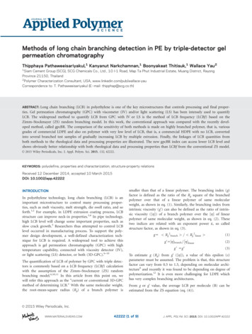
ARTICLEWILEYONLINELIBRARY.COM/APPweight region, as shown in Figure 4(a) for Tests 1 and 2 ofrepeat injections of a same sample. When the SCB correctionwas done for these two plots, the data from Test 2 can beshifted to the linear reference with much lower SCB number,resulting in higher LCBf. If the uncorrected data were used andthe low-cutoff limit was fixed at log M equal to 4.5, both datawould yield the same LCBf. However, there were some errorsremaining from both fluctuating ends.To reduce this fluctuation, much better experimental IV signalis needed. The type of IV was changed to be the capillary bridgeIV with delay volume (Polymer Char, Spain) which providedmore stable baseline and better signal to noise ratio. The previous type was a capillary bridge IV with the diluting volume(Polymer Char, Spain). The LCBf from IV of the new IV forLD-1 provided much less error for corrected and not correctedSCB method, 9.6 and 5.9%, respectively. The curves from thenew Type IV are much smoother as shown in Figure 4(b).Figure 6. (a) Mark–Houwink and (b) conformation plots from online IVand LS detectors of HDPE with multiple extrusions. [Color figure can beviewed in the online issue, which is available at wileyonlinelibrary.com.]From the IV data, the LCBf can be calculated without SCB correction to give the LCBf average around 1.6 with much lesserror (reduce from 29.3 to 9.4%).A parallel shift between the two Log [g] lines in the Mark–Houwink plot is generally considered due to the presence of SCB inthe branched sample. Rightly or wrongly, this has been the basefor the commonly accepted practice in the GPC field to correctfor SCB effect in studying polymer LCB. This correction for theSCB effect can be applied in the commercial GPC software byentering the number of SCBs/1000C to adjust the [g] curve ofan unknown sample iteratively until it is superimposed to thelow-molecular weight region of the [g] line of linear reference.Aside from the conventional SCB correction mentioned above,the SCB can be corrected better today with the advent of thenew online dual-wavelength IR detector. The short chainbranching results can be obtained from the composition calculation when such an IR detector is used. An example of such aresult is shown in Figure 3(a).The sources of error in the conventional method of SCB correction in GPC are from the raw data fluctuation at low-molecularWWW.MATERIALSVIEWS.COMSensitivity of gpcBR and LCBf at Low Level of LCB—TheLow LCB Case of the Janzen–Colby Plot15In this part of our study, a linear commercial HDPE wasselected and passed through the extruder with multiple cycles togradually generate LCB in each cycle. Prior to LCB analysis, themolecular weight distribution of five samples, that is, the original sample, plus the 2nd, 4th, 6th, and 8th cycles’ samples, areplotted and shown in Figure 5. The MMD of all samples arenot significantly different. The weight average molecular weight,MW, from IR detector of the 2nd to 8th cycles were slightlyreduced from that of the original sample, while MZ of theseextruded samples significantly decreased from 1.8 3 106 (original) to 0.6 3 106 g mol21 (the 8th cycle). That means the multiple extrusions affected mostly on the high molecular weightpart of the polymer sample.Interestingly, for multiple extrusion HDPE, the MI decreaseswith increasing extrusion cycles as shown in Figure 5(b). Thisdecrease in MI, meaning an increase in melt viscosity, wouldnot have been intuitively anticipated in view of the decreasingGPC MW and MZ values with increasing extrusion cycles shownin Figure 5(a). Such correlation, however, is exactly what oneshould expect when low level of LCB is generated during meltFigure 7. Increment of gpcBR of each molecular weight fraction withextrusion cycles. [Color figure can be viewed in the online issue, which isavailable at wileyonlinelibrary.com.]42222 (5 of 9)J. APPL. POLYM. SCI. 2015, DOI: 10.1002/APP.42222
ARTICLEWILEYONLINELIBRARY.COM/APPFigure 8. Increasing of LCB; (a) gpcBR, (b) LCBf (IV), and (c) LCBf (LS) of the whole sample with more extrusion cycles. [Color figure can be viewedin the online issue, which is available at wileyonlinelibrary.com.]extrusion at high temperature, alongside with the concurrentchain-scission processes of the polymer molecules. With thepresence of low level of LCB, the melt viscosity of the polymerincreases significantly according to Janzen–Colby plot.15 Furthermore, confirmation of this LCB presence in these samples isprovided by the 3D-GPC results discussed below.Figure 9. Increasing of LCB; (a) gpcBR, (b) LCBf (IV), and (c) LCBf (LS) at high-molecular weight fraction with more extrusion cycles. [Color figurecan be viewed in the online issue, which is available at 2 (6 of 9)J. APPL. POLYM. SCI. 2015, DOI: 10.1002/APP.42222
ARTICLEWILEYONLINELIBRARY.COM/APPFigure 10. Relationship between LCBi and (a) gpcBR, (b) LCBf (IV), and (c) LCBf (LS). [Color figure can be viewed in the online issue, which is available at wileyonlinelibrary.com.]From IV and LS online detectors, the Mark–Houwink plot andconformation plot can be obtained. Both plots in Figure 6 showthat the more extrusion cycles, the more deviation from linearreference, indicating more LCB.From 3D-GPC data, gpcBR and LCBf can be calculated from IVand LS results. From the option offered in the commercial GPCR software, gpcBR can be calculated for each of the fourOneVseparate molecular weight fractions across the sample MWD.Figure 7 shows that gpcBR changed significantly in the highestmolecular weight fraction, Fraction 4, among the five test samples, in the exact trend expected of the increasing LCB levels.This can imply that the high-molecular weight polymer gradu-Figure 11. Schematic drawing of Neck-in measurement in extrusion coating process. [Color figure can be viewed in the online issue, which isavailable at wileyonlinelibrary.com.]WWW.MATERIALSVIEWS.COMally turn into LCB polymer as introduction of heating andshearing in multiple extrusion experiment. The gpcBR values ofthe first fraction of the test samples were quite noisy and notshown here. This is expected because of the usual limitations ofLS and viscosity detection for low-molecular weight polymer.Likewise, LCBf from IV and LS were calculated from 3D-GPCdata. To observe the repeatability of these indices, gpcBR, LCBf(IV), and LCBf (LS) of the original sample and samples fromeven cycles were tested repeatedly with non-consecutive runs by3D-GPC. Figure 8(a) illustrates the increasing of LCB withincreasing gpcBR of the whole sample with very low deviation.The level of LCB in the starting sample and the second extrusioncycle’s sample, and also with the three samples of more extrusioncycles, can be well differentiated. Nevertheless, LCBf from both IVand LS cannot definitely distinguish the adjacent cycles, especiallyfor earlier cycles (0 and 2). This experiment shows that gpcBRcan access lower level of long chain branch in 3D-GPC with morereliable results than the conventional LCBf-ZS method.With the advantage of GPC technology that offers the ability toaccess and process data within any molecular weight region ofinterest, the LCB indices can be determined in selected regions.In this study, since LCB was expected to be generated mostly inthe high molecular weight region, therefore, the gpcBR andLCBf in this fraction were calculated and re-plotted here versusthe number of extrusion cycles in Figure 9. The gpcBR resultsat high-molecular weight region [blue squares in Figure 9(a)]can even more clearly separate all test samples apart, as compared with Figure 8(a) for the whole sample. Remarkably,thanks to the GPC advantage of focusing only on the high-42222 (7 of 9)J. APPL. POLYM. SCI. 2015, DOI: 10.1002/APP.42222
ARTICLEWILEYONLINELIBRARY.COM/APPFigure 12. Long chain branching and neck-in relationship (a) gpcBR, (b) LCBf (IV), and (c) LCBf (LS). [Color figure can be viewed in the online issue,which is available at wileyonlinelibrary.com.]molecular weight region, even the variation of LCBf from bothIV and LS detector were also now significantly improved. Nevertheless, the LCBf of the 2nd cycle sample was still unable to bedifferentiated from the original sample.Comparison of LCB from 3D-GPC and Rheology—The HighLCB Case of the Janzen–Colby Plot15Besides 3D-GPC, another widely used method to determineLCB is rheology.15,17–19 Here, the comparison between the LCBfrom 3D-GPC and the rheology was reported. The rheologyLCB index, called LCBi, is defined in the following equation.g0;branchLCBi5(7)g0;linearwhere g0,branch is the measured zero shear viscosity of the branchedsample, and g0,linear is the zero shear viscosity of the linear polymerwhich has same GPC measured backbone MW,CC as the branchedpolymer, calculated from g0 5 2.29 3 10215MW3.65.20In this part, the relationships between rheology LCBi and theLCB measurement from 3D-GPC, that is, gpcBR, LCBf (IV),and LCBf (LS) were illustrated. This test was done on the sameset of LDPE samples used in “Polymer structure property relationship—relationship of LCB and processing properties” belowfor the coating neck-in test. The plot between gpcBR and LCBishown in Figure 10(a) provided the best linear fit. AlthoughLCBf from both IV and LS in Figure 10(b and c), respectively,shows poor correlation with LCBi, they provide the same trendas gpcBR that is LCBi decreases with increasing LCB from 3DGPC. This trend of decreasing LCBi with increasing LCB forLDPE is the expected result according to the well-known Janzen–Colby plot of predicting LCB effect on rheology for polymers with very high level of LCB.15WWW.MATERIALSVIEWS.COMBut, due to the excessive scattering of the LCBi plot versus LCBfdata, the predictability of melt viscosity property of polymersample from GPC-LCBf measurement is practically all lost,non-existing any more for all practical considerations. This hasbeen the problem commonly faced in studies attempting toestablish correlation of GPC determined LCB results with polymer rheological properties. The use of gpcBR suggested in thiswork should help to provide an improvement in such studies inthe future.Knowing the high precision value of the gpcBR results as demonstrated in “Sensitivity of gpcBR and LCBf at low level ofLong chain branching—The low LCB case of the Janzen-Colbyplot” above on the HDPE extrusion study, the most of the scatter of the data points in Figure 10(a) could be caused more significantly from the variations in the LCBi measurement thanthat from gpcBR.Polymer Structure Property Relationship—Relationship ofLCB and Processing PropertiesLCB is one of the most important microstructures that influences the processing properties, especially on Neck-in level.3,4 Inthis part of our study, various grades of LDPE have beenselected to verify the relationship between Neck-in and LCB.The processing test was investigated by using a laboratory extrusion coating (Collin, Germany) with fixing line speed of 4 and12 m min21. The neck-in value was measured at the distance of10 cm from die lip as a difference between the melt width andthe die width as shown in Figure 11.Figure 12(a) presents the linear relationship between Neck-inand gpcBR with R-square greater than 0.97. Neck-in value isreduced with higher gpcBR, which represents higher long chain42222 (8 of 9)J. APPL. POLYM. SCI. 2015, DOI: 10.1002/APP.42222
ARTICLEWILEYONLINELIBRARY.COM/APPbranching. Low neck-in value indicates good processing performance. Similarly the LCBf from IV and LS also shows linearrelationship with Neck-in as shown in Figure 12(b,c), but withlower R-square than gpcBR where both results of gpcBRand LCBf values are calculated from exactly the same set ofdata files.4. Kouda, S. Polym. Eng. Sci. 2008, 48, 1094.5. Mehta, S. D.; Reinking, M. K.; Joseph, S.; Garrison, P. J.;Lewis, E. O.; Schwab, T. J.; Yau, W. W. Pub. No. US2009/0304966, United State, 2009.6. Grcev, S.; Schoenmakers, P.; Iedema, P. Polymer 2004, 45, 39.7. Stadler, F. J. Rheol. Acta 2012, 51, 821.CONCLUSIONS8. Suarez, I.; Coto, B. Eur. Polym. J. 2013, 49, 492.GPC with online IV and LS detector is an effective tool todetermine LCB ranging from very low to very high level. ThegpcBR method provides more reliable results than the methodof LCBf based on ZS model. This is shown in the experimentwith slightly increasing LCB in HDPE with multiple extrusioncycles. We showed here that gpcBR can access lower LCB levelthan the current LCBf approach with results calculated from thesame experimental data files, (under exactly the same instrumental and measurement conditions). Moreover, the gpcBRresults showed a nice correlation to the rheological LCBi measurement, and also to the processing properties, such as theneck-in data in LDPE coating process, with higher r-square correlation index value than that of the LCBf results.9. Tackx, P.; Tacx, J. C. J. F. Polymer 1998, 39, 3109.We gratefully thank the technical service team (Ms. SalinthipPrathuangsuksri and Ms. Pimnattha Ang-atikarnkul) from SCGPlastics Co., Ltd. for their information and effort on LDPEextrusion coating experiment and SCG Chemical Co., Ltd. forthe financial support.10. Yu, Y.; DesLauriers, P. J.; Rohlfing, D. C. Polymer 2005, 46,5165.11. Zimm, B. H.; Stockmayer, W. H. J. J. Chem. Phys. 1949, 17,1301.12. Kratochv ıl, P.; Netopil ık, M. Eur. Polym. J. 2014, 51, 177.13. Enos, C. T.; Rufener, K.; Merrick-Mack, J.; Yau, W. WaterInternational GPC Symposium Proceedings, Baltimore, MD,6–12 Jun 2013; 2003.14. Enos, C. T.; Yau, W. PITTCON (Pittsburgh Conference)2004 preceeding, Chicago, IL, 2004.15. Janzen, J.; Colby, R. H. J. Mol. Struct. 1999, 485, 569.16. Podzimek, S. Light Scattering, Size Exclusion Chromatography and Asymmetric Flow Field Flow Fractionation—Powerful Tools for the Characterization of Polymers, Proteins; Nanoparticles; Wiley: Hoboken, New Jersey, 2011.17. Wood-Adams, P. M.; Dealy, J. M.; deGroot, A. W.; Redwine,O. D. Macromolecules 2000, 33, 7489.18. Larson, R. G. Macromolecules 2001, 34, 4556.19. Stadler, F. J.; Karimkhani, V. Macromolecules 2011, 44, 5401.REFERENCES1. Barroso, V. C.; Maia, J. M. Polym. Eng. Sci. 2005, 45, 984.2. Yan, D.; Wang, W.-J.; Zhu, S. Polymer 1999, 40, 1737.3. Honkanen, A.; Bergstr om, C.; Laiho, E. Polym. Eng. Sci.1978, 18, 985.WWW.MATERIALSVIEWS.COM20. Karjala, T. P.; Sammler, R. L.; Mangnus, M. A.; Hazlitt, L.G.; Johnson, M. S.; Hagen, J. C. M.; Huang, J. W. L.;Reichek, Detection of low levels of long-chain branchingin polyolefins
For branched polymer, we selected a commercial LDPE as a highly branched polymer (LD-1), and a commercial HDPE with no LCB (HD-1), which is transformed into several branched test samples of gradually increasing LCB by multiple extrusion. LDPE sample was measured 10 times on a high temperature GPC instrument with triple detectors (Polymer Char .