Transcription
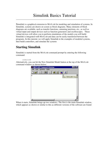
Simulink Basics TutorialSimulink is a graphical extension to MATLAB for modeling and simulation of systems. InSimulink, systems are drawn on screen as block diagrams. Many elements of blockdiagrams are available, such as transfer functions, summing junctions, etc., as well asvirtual input and output devices such as function generators and oscilloscopes. Thesevirtual devices will allow you to perform simulations of the models you will build.Simulink is integrated with MATLAB and data can be easily transferred between theprograms. In this tutorial, we will apply Simulink to the examples of modeled systems,then build controllers, and simulate the systemsStarting SimulinkSimulink is started from the MATLAB command prompt by entering the followingcommand:simulinkAlternatively, you can hit the New Simulink Model button at the top of the MATLABcommand window as shown below:When it starts, Simulink brings up two windows. The first is the main Simulink window,which appears as shown or similar to this as different versions of the software are found:
The second window is a blank, untitled, model window. This is the window into which anew model can be drawn.Model FilesIn Simulink, a model is a collection of blocks which, in general, represents a system. Inaddition, to drawing a model into a blank model window, previously saved model filescan be loaded either from the File menu or from the MATLAB command prompt. As afirst exercise we will be building a model.You can open a file in Simulink by entering the following command in the MATLABcommand window. (Alternatively, you can load this file using the Open option in theFile menu in Simulink, or by hitting Ctrl O in Simulink.)File name.mdlFor our purposes we will create the following model in simulink. A new model can becreated by selecting New from the File menu in any Simulink window (or by hittingCtrl N). Using the information below, create the following model.Basic ElementsThere are two major classes of items in Simulink: blocks and lines. Blocks are used togenerate, modify, combine, output, and display signals. Lines are used to transfer signalsfrom one block to another.
BlocksThere are several general classes of blocks: Sources: Used to generate various signalsSinks: Used to output or display signalsDiscrete: Linear, discrete-time system elements (transfer functions, state-spacemodels, etc.)Linear: Linear, continuous-time system elements and connections (summingjunctions, gains, etc.)Nonlinear: Nonlinear operators (arbitrary functions, saturation, delay, etc.)Connections: Multiplex, Demultiplex, System Macros, etc.Blocks have zero to several input terminals and zero to several output terminals. Unusedinput terminals are indicated by a small open triangle. Unused output terminals areindicated by a small triangular point. The block shown below has an unused inputterminal on the left and an unused output terminal on the right.LinesLines transmit signals in the direction indicated by the arrow. Lines must always transmitsignals from the output terminal of one block to the input terminal of another block. Onexception to this is a line can tap off of another line, splitting the signal to each of twodestination blocks, as shown. Lines can never inject a signal into another line; lines mustbe combined through the use of a block such as a summing junction.A signal can be either a scalar signal or a vector signal. For Single-Input, Single-Outputsystems, scalar signals are generally used. For Multi-Input, Multi-Output systems, vectorsignals are often used, consisting of two or more scalar signals. The lines used to transmitscalar and vector signals are identical. The blocks on either end of the line determine thetype of signal carried by the line.
Simple ExampleThe simple model (from the model file section) consists of three blocks: Step, TransferFcn, and Scope. The Step is a source block from which a step input signal originates.This signal is transferred through the line in the direction indicated by the arrow to theTransfer Function linear block. The Transfer Function modifies its input signal andoutputs a new signal on a line to the Scope. The Scope is a sink block used to display asignal much like an oscilloscope.There are many more types of blocks available in Simulink, some of which will bediscussed later. Right now, we will examine just the three we have used in the simplemodel.Modifying BlocksA block can be modified by double-clicking on it. For example, if you double-click onthe "Transfer Fcn" block in the simple model, you will see the following dialog box.This dialog box contains fields for the numerator and the denominator of the block'stransfer function. By entering a vector containing the coefficients of the desirednumerator or denominator polynomial, the desired transfer function can be entered.For example, to change the denominator to s2 2s 4, enter the following into thedenominator field:[1 2 4]
and hit the close button, the model window will change to the following,which reflects the change in the denominator of the transfer function.The "step" block can also be double-clicked, bringing up the following dialog box.The default parameters in this dialog box generate a step function occurring at time 1sec, from an initial level of zero to a level of 1. (in other words, a unit step at t 1). Eachof these parameters can be changed. Close this dialog before continuing.The most complicated of these three blocks is the "Scope" block. Double clicking on thisbrings up a blank oscilloscope screen.When a simulation is performed, the signal which feeds into the scope will be displayed
in this window. Detailed operation of the scope will not be covered in this tutorial. Theonly function we will use is the autoscale button, which appears as a pair of binoculars inthe upper portion of the window.Running SimulationsTo run a simulation, we will work with the following model. Using the techniquesdeveloped above creates the following model:Before running a simulation of this system, first open the scope window by doubleclicking on the scope block. Then, to start the simulation, either select Start from theSimulation menu (as shown below) or hit Ctrl-T in the model window.The simulation should run very quickly and the scope window will appear as shownbelow.Note that the simulation output (shown in yellow) is at a very low level relative to the
axes of the scope. To fix this, hit the autoscale button (binoculars), which will rescale theaxes as shown below.Note that the step response does not begin until t 1. This can be changed by doubleclicking on the "step" block. Now, we will change the parameters of the system andsimulate the system again. Double-click on the "Transfer Fcn" block in the modelwindow and change the denominator to[1 20 400]Re-run the simulation (hit Ctrl-T) and you should see what appears as a flat line in thescope window. Hit the autoscale button, and you should see the following in the scopewindow.Notice that the autoscale button only changes the vertical axis. Since the new transferfunction has a very fast response, it compressed into a very narrow part of the scopewindow. This is not really a problem with the scope, but with the simulation itself.Simulink simulated the system for a full ten seconds even though the system had reachedsteady state shortly after one second.To correct this, you need to change the parameters of the simulation itself. In the modelwindow, select Parameters from the Simulation menu. You will see the following
dialog box.There are many simulation parameter options; we will only be concerned with the startand stop times, which tell Simulink over what time period to perform the simulation.Change Start time from 0.0 to 0.8 (since the step doesn't occur until t 1.0. Change Stoptime from 10.0 to 2.0, which should be only shortly after the system settles. Close thedialog box and rerun the simulation. After hitting the auto-scale button, the scopewindow should provide a much better display of the step response as shown below.Building SystemsIn this section, you will learn how to build systems in Simulink using the building blocksin Simulink's Block Libraries. You will build the following system.
First you will gather all the necessary blocks from the block libraries. Then you willmodify the blocks so they correspond to the blocks in the desired model. Finally, you willconnect the blocks with lines to form the complete system. After this, you will simulatethe complete system to verify that it works.Gathering BlocksFollow the steps below to collect the necessary blocks: Create a new model (New from the File menu or Ctrl-N). You will get a blankmodel window.
Double-click on the Sources icon in the main Simulink window.This opens the Sources window which contains the Sources Block Library.Sources are used to generate signals. Click here for more information on blocklibraries.
Drag the Step block from the sources window into the left side of your modelwindow. Double-click on the Linear icon in the main Simulink window to open the LinearBlock Library window.Drag the Sum, Gain, and two instances of the Transfer Fcn (drag it two times)into your model window arranged approximately as shown below. The exactalignment is not important since it can be changed later. Just try to get the correctrelative positions. Notice that the second Transfer Function block has a 1 after itsname. Since no two blocks may have the same name, Simulink automaticallyappends numbers following the names of blocks to differentiate between them. Double-click on the Sinks icon in the main Simulink window to open the Sinkswindow.
Drag the Scope block into the right side of your model window.Modify BlocksFollow these steps to properly modify the blocks in your model. Double-click your Sum block. Since you will want the second input to besubtracted, enter - into the list of signs field. Close the dialog box.Double-click your Gain block. Change the gain to 2.5 and close the dialog box.Double-click the leftmost Transfer Function block. Change the numerator to [1 2]and the denominator to [1 0]. Close the dialog box.Double-click the rightmost Transfer Function block. Leave the numerator [1], butchange the denominator to [1 2 4]. Close the dialog box. Your model shouldappear as:Change the name of the first Transfer Function block by clicking on the words"Transfer Fcn". A box and an editing cursor will appear on the block's name asshown below. Use the keyboard (the mouse is also useful) to delete the existingname and type in the new name, "PI Controller". Click anywhere outside the
name box to finish editing. Similarly, change the name of the second Transfer Function block from "TransferFcn1" to "Plant". Now, all the blocks are entered properly. Your model shouldappear as:Connecting Blocks with LinesNow that the blocks are properly laid out, you will now connect them together. Followthese steps. Drag the mouse from the output terminal of the Step block to the upper (positive)input of the Sum block. Let go of the mouse button only when the mouse is righton the input terminal. Do not worry about the path you follow while dragging, theline will route itself. You should see the following.
The resulting line should have a filled arrowhead. If the arrowhead is open, asshown below, it means it is not connected to anything. You can continue the partial line you just drew by treating the open arrowhead asan output terminal and drawing just as before. Alternatively, if you want toredraw the line, or if the line connected to the wrong terminal, you should deletethe line and redraw it. To delete a line (or any other object), simply click on it toselect it, and hit the delete key.Draw a line connecting the Sum block output to the Gain input. Also draw a linefrom the Gain to the PI Controller, a line from the PI Controller to the Plant, and a
line from the Plant to the Scope. You should now have the following. The line remaining to be drawn is the feedback signal connecting the output of thePlant to the negative input of the Sum block. This line is different in two ways.First, since this line loops around and does not simply follow the shortest (rightangled) route so it needs to be drawn in several stages. Second, there is no outputterminal to start from, so the line has to tap off of an existing line.To tap off the output line, hold the Ctrl key while dragging the mouse from thepoint on the existing line where you want to tap off. In this case, start just to theright of the Plant. Drag until you get to the lower left corner of the desiredfeedback signal line as shown below.Now, the open arrowhead of this partial line can be treated as an output terminal.
Draw a line from it to the negative terminal of the Sum block in the usual manner. Now, you will align the blocks with each other for a neater appearance. Onceconnected, the actual positions of the blocks does not matter, but it is easier toread if they are aligned. To move each block, drag it with the mouse. The lineswill stay connected and re-route themselves. The middles and corners of lines canalso be dragged to different locations. Starting at the left, drag each block so thatthe lines connecting them are purely horizontal. Also, adjust the spacing betweenblocks to leave room for signal labels. You should have something like: Finally, you will place labels in your model to identify the signals. To place alabel anywhere in your model, double click at the point you want the label to be.Start by double clicking above the line leading from the Step block. You will get ablank text box with an editing cursor as shown below
Type an r in this box, labeling the reference signal and click outside it to endediting.Label the error (e) signal, the control (u) signal, and the output (y) signal in thesame manner. Your final model should appear as:To save your model, select Save As in the File menu and type in any desiredmodel name. The completed model can be found here.SimulationNow that the model is complete, you can simulate the model. Select Start from theSimulation menu to run the simulation. Double-click on the Scope block to view its
output. Hit the autoscale button (binoculars) and you should see the following.Taking Variables from MATLABIn some cases, parameters, such as gain, may be calculated in MATLAB to be used in aSimulink model. If this is the case, it is not necessary to enter the result of the MATLABcalculation directly into Simulink. For example, suppose we calculated the gain inMATLAB in the variable K. Emulate this by entering the following command at theMATLAB command prompt.K 2.5This variable can now be used in the Simulink Gain block. In your simulink model,double-click on the Gain block and enter the following in the Gain field.KClose this dialog box. Notice now that the Gain block in the Simulink model shows thevariable K rather than a number.
Now, you can re-run the simulation and view the output on the Scope. The result shouldbe the same as before.Now, if any calculations are done in MATLAB to change any of the variable used in theSimulink model, the simulation will use the new values the next time it is run. To try this,in MATLAB, change the gain, K, by entering the following at the command prompt.K 5
Start the Simulink simulation again, bring up the Scope window, and hit the auto-scalebutton. You will see the following output which reflects the new, higher gain.Besides variable, signals, and even entire systems can be exchanged between MATLABand Simulink. For more information see belowSimulink Basics Tutorial - Interaction WithMATLABDefining Block Parameters Using MATLAB VariablesExchanging Signals With MATLABExtracting Models From Simulink Into MATLABWe will examine three of the ways in which Simulink can interact with MATLAB. Block parameters can be defined from MATLAB variable.Signals can be exchanged between Simulink and MATLAB.Entire systems can be extracted from Simulink into MATLAB.Block Parameters from MATLAB VariablesOften, a controller will be designed in MATLAB and verified in a Simulink model.Normally, numerical parameters such as gains and controller transfer functions areentered into simulink manually by entering the numbers in the block dialog boxes. Rather
than enter numbers directly, it is possible to use MATLAB variable in Simulink blockdialog boxes.For example, bring up the Simulink model built in the Basics tutorial (or click here todownload it.)In this case, the complete controller transfer function is:s 22.5 ----sSuppose this transfer function were generated by some computation in MATLAB. In thiscase, there would most likely be three variable, the numerator polynomial, thedenominator polynomial, and the gain. Enter the following commands in MATLAB togenerate these variable.K 2.5num [1 2]den [1 0]These variable can now be used in the blocks in Simulink. In your simulink model,double-click on the Gain block. Enter the following in the Gain field.KClose this dialog box. Notice now that the Gain block in the Simulink model shows thevariable K rather than a number.
Double-click on the PI Controller block. Enter the following into the Numerator field.numEnter the following into the Denominator field.denClose this dialog box. Notice now that the PI Controller block shows the variable numand den (as functions of s) rather than an explicit transfer function.
You can simulate the model with the MATLAB variable parameters. Select Start from theSimulation menu to run the simulation. Double-click on the Scope block to view itsoutput. Hit the autoscale button (binoculars) and you should see the following.Now, if any calculations are done in MATLAB to change any of the variable used in theSimulink model, the simulation will use the new values the next time it is run. To try this,in MATLAB, change the gain, K, by entering the following at the command prompt.K 5Start the Simulink simulation again, bring up the Scope window, and hit the autoscalebutton. You will see the following output which reflects the new, higher gain.To download the model with MATLAB variable parameters, click here.Exchanging Signals with MATLABSometimes, we would like to use the results of a Simulink simulation in the MATLABcommand window for further calculations and plotting. Less often, we would like togenerate signals in MATLAB which we then use as inputs in a Simulink model. Thesetasks are accomplished through the use of the To Workspace Sink Block and the From
Workspace Source Block. We will only transfer signals from Simulink to MATLAB.Doing the reverse is a very similar process.The To Workspace Sink Block saves a signal as a vector in the MATLAB Workspace.Open the model which you used previously in this tutorial or click here to download themodel. Be sure that the variable K ( 5), num ( [1 2]), and den ( [1 0]) are defined inMATLAB.Supposewe would like to use both the output signal and the control signal for calculations inMATLAB. We will save these two variables as well as a time signal from our Simulinkmodel. First, you need to generate a time signal. Open the Sources window by doubleclicking the Sources icon in the main Simulink window. Drag the Clock block from theSources window to the lower portion of your Simulink model.Now, open the Sinks window and drag three instances of the To Workspace block to yourSimulink window, arranged approximately as shown below.
Before connecting these blocks to the rest of your system, first you will name the variableto which they output. The lower To Workspace block will output the time signal to theMATLAB variable. Double-click on this block and enter the following in the VariableName field.tClose the dialog box. Notice that the lower To Workspace block shows a t.
The ToWorkspace block near the Plant block will output the control signal to the MATLABvariable u. Edit this block to output to the variable u. The last To Workspace block willoutput the output signal to the MATLAB variable y. Edit this block to output to thevariable y. Also, for better clarity, change the labels (by clicking on the exiting labels "ToWorkspace") of these blocks to "time", "control", and "output".Now, you will connect these blocks to the rest of your system. Draw a line from theClock block to the time (t) block. Tap a line off of the control signal (the line between thePI Controller block and the Plant block) and connect it to the control (u) block.Remember, to tap off an existing line, hold the Ctrl key while drawing the line. Tap a lineoff the output signal line (the line which enters the Scope block) and connect it to theoutput (y) block. Your system should appear as follows.
Start the simulation (Start from the Simulation menu). You can still view the output inthe Scope window (remember autoscale).You can now examine the outputted variable in the MATLAB window. Plot u and y vs. tby entering the following command.plot(t,u,t,y);Note that it is important to plot each of these variables against the time vector generatedby Simulink, since the time between elements in the signal vectors u and y may beunequal, particularly near a discontinuity such as the step input. Your plot of u (blue) andy (green) should appear as follows.
To download the model with outputs to MATLAB variable, click here.Extracting Models From Simulink into MATLABSometimes, we may build a complicated model in simulink and would like to deriveeither a transfer function or a state space model of the entire system. In order to do this,you first need to define the input and output signals of the model to be extracted. Thesevirtual signals can be any signal in a model, for example, if we can generate an input-tooutput transfer function or a disturbance-to-error transfer function. These signals aredefined using the In and Out Connection Blocks.Once the input/output model is defined, the Simulink model must be saved to a .mdl file.This file is then referenced in the MATLAB command window by the linmod command.To demonstrate this, bring up your model from the previous section of this tutorial (orclick here to download it). Be sure that the variable K ( 5), num ( [1 2]), and den ( [10]) are defined in MATLAB.
You will be extracting a closed-loop reference-to-output model. Therefore, The virtualinput will be put in place of the step input to the system. First, delete the Step block (clickon it and hit the delete key). The previous line will remain with an open input terminalwhere it used to connect to the Step. Open the Connections window from the mainSimulink window. Drag an In Block from the Connections window to your modelwindow in place of the Step block you just deleted. Move the In block until the outputterminal of the In block touches the open input terminal of the left over line. The lineshould attach to the In block.The virtual output does not need to replace an existing block - the signal can be tappedoff an existing line. Drag an Out block from the Connections window and place it justabove the Scope block. Tap a line off the output signal (hold Ctrl) and connect it to theout block.
Now, save this model under a new name. Call it mymodel.mdl. You can download aversion here.At the MATLAB prompt, enter the following command to extract a state-space modelfrom your model file.[A,B,C,D] linmod('mymodel')You should see the following output.A -210-90-520010B 505C 0D 0This can, of course, be converted to a transfer function with the following command.[numcl,dencl] ss2tf(A,B,C,D)You should get the following output.numcl 0dencl 05.000010.0000
1.00002.00009.000010.0000To verify that the model transfered properly, you can obtain a step response of theextracted model.step(numcl,dencl)You should see the following plot which is similar to the previous Simulink Scopeoutput.The modeling information is continued below:Simulink Modeling TutorialTrain systemFree body diagram and Newton's lawModel ConstructionRunning the ModelObtaining MATLAB ModelIn Simulink, it is very straightforward to represent a physical system or a model. Ingeneral, a dynamic system can be constructed from just basic physical laws. We willdemonstrate through an example.
Train systemIn this example, we will consider a toy train consisting of an engine and a car. Assumingthat the train only travels in one direction, we want to apply control to the train so that ithas a smooth start-up and stop, along with a constant-speed ride.The mass of the engine and the car will be represented by M1 and M2, respectively. Thetwo are held together by a spring, which has the stiffness coefficient of k. F represents theforce applied by the engine, and the Greek letter, mu (which will also be represented bythe letter u), represents the coefficient of rolling friction.Free body diagram and Newton's lawThe system can be represented by following Free Body Diagrams.From Newton's law, you know that the sum of forces acting on a mass equals the masstimes its acceleration. In this case, the forces acting on M1 are the spring, the friction andthe force applied by the engine. The forces acting on M2 are the spring and the friction.In the vertical direction, the gravitational force is canceled by the normal force applied bythe ground, so that there will be no acceleration in the vertical direction. We will begin toconstruct the model simply from the expressions:Sum(forces on M1) M1*x1''Sum(forces on M1) M1*x1''Constructing The ModelThis set of system equations can now be represented graphically, without furthermanipulation. First, we will construct two copies (one for each mass) of the expressionssum F Ma or a 1/M*sum F. Open a new model window, and drag two Sum blocks(from the Linear library), one above the other. Label these Sum blocks "Sum F1" and"Sum F2".
The outputs of each of these Sum blocks represents the sum of the forces acting on eachmass. Multiplying by 1/M will give us the acceleration. Drag two Gain blocks into yourmodel and attach each one with a line to the outputs of the Sum blocks.These Gain blocks should contain 1/M for each of the masses. We will be taking thesevariable as M1 and M2 from the MATLAB environment, so we can just enter the variablein the Gain blocks. Double-click on the upper Gain block and enter the following into theGain field.1/M1Similarly, change the second Gain block to the following.1/M2Now, you will notice that the gains did not appear in the Gain blocks, and just "-K-"shows up. This is because the blocks are two small on the screen to show 1/M2 inside thetriangle. The blocks can be resized so that the actual gain can be seen. To resize a block,
select it by clicking on it once. Small squares will appear at the corners. Drag one ofthese squares to stretch the block.When the Gain blocks are of sufficient size to display the actual gains, re-align them withthe signal line output from the Sum blocks. Also, label these two Gain blocks "a1" and"a2".The outputs of these gain blocks are the accelerations of each of the masses. We areinterested in both the velocities and the positions of the masses. Since velocity is theintegral of acceleration, and position is the integral of velocity, we can generate thesesignals using integrator blocks. Drag two integrator blocks into your model for each ofthe two accelerations. Connect them with lines in two chains as shown below. Label theseintegrators "v1", "x1", "v2", and "x2" since these are the signals these integrators willgenerate.
Now, drag two Scopes from the Sinks library into your model and connect them to theoutputs of these integrators. Label them "View x1" and "View x2".Now we are ready to add in the forces acting on each mass. First, you need to adjust theinputs on each Sum block to represent the proper number (we will worry about the signlater) of forces. There are a total of 3 forces acting on M1, so change the Sum F1 block'sdialog box entry to:
There are only 2 forces acting on M2, so we can leave Sum F1 alone for now.The first force acting on M1 is just the input force, F. Drag a Signal Generator block fromthe Sources library and connect it to the uppermost input of the Sum F1 block. Label theSignal Generator "F".The next force acting on M1 is the friction force. This force is equal to:F friction 1 mu*g*M1*v1To generate this force, we can tap off the velocity signal and multiply by a gain,mu*g*M1. Drag a Gain block into your model window. Tap off the line coming from thev1 integrator and connect it to the input of the Gain block (draw this line in several stepsif necessary). Connect the output of the Gain block to the second input of Sum F1.Change the gain of this gain block to the following.mu*g*M1
Resize the Gain block to display the gain and label the gain block Friction 1.This force, however, acts in the negative x1-direction. Therefore, it must come into theSum F1 block with negative sign. Change the list of signs of Sum F1 to - The last force acting on M1 is the spring force between masses. This is equal to:k*(x1-x2)First, we need to generate (x1-x2) which we can then multiply by k to generate the force.Drag a Sum block below the rest of your model. Label it "(x1-x2)" and change its list ofsigns to- Since this summation comes from right to left, we need to flip the block around. Selectthe bloc by single-clicking on it and select Flip from the Format menu (or hit Ctrl-F).You should see the following.
Now, tap off the x2 signal and connect it to the negative input of the (x1-x2) Sum block.Tap off the x1 signal and connect it to the positive input. This will cause the lines tocross. Lines may cross, but they are only actually connected where a small block appears(such as at a tap point).Now, we can multiply this position difference by the spring constant to generate thespring force. Drag a Gain block into your model to the left of the Sum blocks. Change it'sva
Simulink Basics Tutorial Simulink is a graphical extension to MATLAB for modeling and simulation of systems. In Simulink, systems are drawn on screen as block diagrams. Many elements of block diagrams are available, such a
