Transcription
COURSE NOTESSTATS 325Stochastic ProcessesDepartment of StatisticsUniversity of Auckland
Contents1. Stochastic Processes1.1 Revision: Sample spaces and random variables . . . . . . . . . . . . . . . . . . .1.2 Stochastic Processes . . . . . . . . . . . . . . . . . . . . . . . . . . . . . . . . .2. Probability2.1 Sample spaces and events . . . . . . . . . . . . . . . . . . .2.2 Probability Reference List . . . . . . . . . . . . . . . . . . .2.3 Conditional Probability . . . . . . . . . . . . . . . . . . . . .2.4 The Partition Theorem (Law of Total Probability) . . . . . .2.5 Bayes’ Theorem: inverting conditional probabilities . . . . .2.6 First-Step Analysis for calculating probabilities in a process2.7 Special Process: the Gambler’s Ruin . . . . . . . . . . . . .2.8 Independence . . . . . . . . . . . . . . . . . . . . . . . . . .2.9 The Continuity Theorem . . . . . . . . . . . . . . . . . . . .2.10 Random Variables . . . . . . . . . . . . . . . . . . . . . . . .2.11 Continuous Random Variables . . . . . . . . . . . . . . . . .2.12 Discrete Random Variables . . . . . . . . . . . . . . . . . . .2.13 Independent Random Variables . . . . . . . . . . . . . . . .3. Expectation and Variance3.1 Expectation . . . . . . . . . . . . . . . . . . . . . . . . . .3.2 Variance, covariance, and correlation . . . . . . . . . . . .3.3 Conditional Expectation and Conditional Variance . . . .3.4 Examples of Conditional Expectation and Variance . . . .3.5 First-Step Analysis for calculating expected reaching times3.6 Probability as a conditional expectation . . . . . . . . . .3.7 Special process: a model for gene spread . . . . . . . . . 4. Generating Functions4.1 Common sums . . . . . . . . . . . . . . . . . . . . . . . . . . . .4.2 Probability Generating Functions . . . . . . . . . . . . . . . . . .4.3 Using the probability generating function to calculate probabilities4.4 Expectation and moments from the PGF . . . . . . . . . . . . . .4.5 Probability generating function for a sum of independent r.v.s . .4.6 Randomly stopped sum . . . . . . . . . . . . . . . . . . . . . . . .747476798182831.
4.74.84.94.104.11Summary: Properties of the PGF . . . . . . . . .Convergence of PGFs . . . . . . . . . . . . . . . .Special Process: the Random Walk . . . . . . . .Defective random variables . . . . . . . . . . . . .Random Walk: the probability we never reach our. . . . . . . . .goal.8990951011055. Mathematical Induction1085.1 Proving things in mathematics . . . . . . . . . . . . . . . . . . . . . . . . . . . . 1085.2 Mathematical Induction by example . . . . . . . . . . . . . . . . . . . . . . . . . 1105.3 Some harder examples of mathematical induction . . . . . . . . . . . . . . . . . 1136. Branching Processes:6.1 Branching Processes . . . . . . . . . . . . .6.2 Questions about the Branching Process . . .6.3 Analysing the Branching Process . . . . . .6.4 What does the distribution of Zn look like?6.5 Mean and variance of Zn . . . . . . . . . . .7. Extinction in Branching Processes7.1 Extinction Probability . . . . . .7.2 Conditions for ultimate extinction7.3 Time to Extinction . . . . . . . .7.4 Case Study: Geometric Branching. . . . . . . . . . . . . . . .Processes.8. Markov Chains8.1 Introduction . . . . . . . . . . . . . . . . . . . . . .8.2 Definitions . . . . . . . . . . . . . . . . . . . . . . .8.3 The Transition Matrix . . . . . . . . . . . . . . . .8.4 Example: setting up the transition matrix . . . . .8.5 Matrix Revision . . . . . . . . . . . . . . . . . . . .8.6 The t-step transition probabilities . . . . . . . . . .8.7 Distribution of Xt . . . . . . . . . . . . . . . . . .8.8 Trajectory Probability . . . . . . . . . . . . . . . .8.9 Worked Example: distribution of Xt and trajectory8.10 Class Structure . . . . . . . . . . . . . . . . . . . .8.11 Hitting Probabilities . . . . . . . . . . . . . . . . .8.12 Expected hitting times . . . . . . . . . . . . . . . .9. Equilibrium9.1 Equilibrium distribution in pictures .9.2 Calculating equilibrium distributions9.3 Finding an equilibrium distribution .9.4 Long-term behaviour . . . . . . . . .9.5 Irreducibility . . . . . . . . . . . . . . . . . . . . . . . . . . . . . . . . . . . . . . . . . . . . . . . . . . . . . . . . . . . . .probabilities. . . . . . . . . . . . . . . . . . .116117119120124128.132. 133. 139. 143. 146.149. 149. 151. 152. 154. 154. 155. 157. 160. 161. 163. 164. 170.174. 175. 176. 177. 179. 183
9.69.79.89.9Periodicity . . . . . . . . . . . . . . . . .Convergence to Equilibrium . . . . . . .Examples . . . . . . . . . . . . . . . . .Special Process: the Two-Armed Bandit.184187188192
Chapter 1: Stochastic Processes4What are Stochastic Processes, and how do they fit in?STATS 310StatisticsSTATS 210Randomness in PatternFoundations ofStatistics and ProbabilityTools for understanding randomness(random variables, distributions)STATS 325ProbabilityRandomness in ProcessStats 210: laid the foundations of both Statistics and Probability: the tools forunderstanding randomness.Stats 310: develops the theory for understanding randomness in pattern: toolsfor estimating parameters (maximum likelihood), testing hypotheses, modellingpatterns in data (regression models).Stats 325: develops the theory for understanding randomness in process. Aprocess is a sequence of events where each step follows from the last after arandom choice.What sort of problems will we cover in Stats 325?Here are some examples of the sorts of problems that we study in this course.Gambler’s RuinYou start with 30 and toss a fair coinrepeatedly. Every time you throw a Head, youwin 5. Every time you throw a Tail, you lose 5. You will stop when you reach 100 or whenyou lose everything. What is the probability thatyou lose everything?Answer: 70%.
5Winning at tennisWhat is your probability of winning a game of tennis,starting from the even score Deuce (40-40), if yourprobability of winning each point is 0.3 and youropponent’s is 0.7?Answer: 15%.qpVENUSAHEAD (A)qVENUSBEHIND (B)pVENUSWINS (W)DEUCE (D)qVENUSLOSES (L)pWinning a lotteryA million people have bought tickets for the weekly lotterydraw. Each person has a probability of one-in-a-millionof selecting the winning numbers. If more than one personselects the winning numbers, the winner will be chosenat random from all those with matching numbers.You watch the lottery draw on TV and your numbers match the winning numbers!!! Only a one-in-a-million chance, and there were only a million players,so surely you will win the prize?Not quite. . .What is the probability you will win?Answer: only 63%.Drunkard’s walkA very drunk person staggers to left and right as he walks along. With eachstep he takes, he staggers one pace to the left with probability 0.5, and onepace to the right with probability 0.5. What is the expected number of paceshe must take before he ends up one pace to the left of his starting point?Arrived!Answer: the expectation is infinite!
6Pyramid selling schemesHave you received a chain letter like this one? Just send 10 to the personwhose name comes at the top of the list, and add your own name to the bottomof the list. Send the letter to as many people as you can. Within a few months,the letter promises, you will have received 77,000 in 10 notes! Will you?Answer: it depends upon the response rate. However, with a fairly realisticassumption about response rate, we can calculate an expected return of 76with a 64% chance of getting nothing!Note: Pyramid selling schemes like this are prohibited under the Fair Trading Act,and it is illegal to participate in them.Spread of SARSThe figure to the right shows the spreadof the disease SARS (Severe AcuteRespiratory Syndrome) through Singaporein 2003. With this pattern of infections,what is the probability that the diseaseeventually dies out of its own accord?Answer: 0.997.
7Markov’s Marvellous Mystery ToursMr Markov’s Marvellous Mystery Tours promises an All-Stochastic Tourist Experience for the town of Rotorua. Mr Markov has eight tourist attractions, towhich he will take his clients completely at random with the probabilities shownbelow. He promises at least three exciting attractions per tour, ending at eitherthe Lady Knox Geyser or the Tarawera Volcano. (Unfortunately he makes nomention of how the hapless tourist might get home from these places.)What is the expected number of activities for a tour starting from the museum?1/32. Cruise1/31/31. Museum1/34. Flying Fox1/31/33. Buried Village1/31/316. Geyser1/35. Hangi11/31/31/37. Helicopter8. Volcano11Answer: 4.2.Structure of the course Probability. Probability and random variables, with special focus onconditional probability. Finding hitting probabilities for stochastic processes. Expectation. Expectation and variance. Introduction to conditional expectation, and its application in finding expected reaching times in stochastic processes. Generating functions. Introduction to probability generating functions, and their applications to stochastic processes, especially the RandomWalk. Branching process. This process is a simple model for reproduction.Examples are the pyramid selling scheme and the spread of SARS above.
8 Markov chains. Almost all the examples we look at throughout thecourse can be formulated as Markov chains. By developing a single unifying theory, we can easily tackle complex problems with many states andtransitions like Markov’s Marvellous Mystery Tours above.The rest of this chapter covers: quick revision of sample spaces and random variables; formal definition of stochastic processes.1.1 Revision: Sample spaces and random variablesDefinition: A random experiment is a physical situation whose outcome cannotbe predicted until it is observed.Definition: A sample space, Ω, is a set of possible outcomes of a random experiment.Example:Random experiment: Toss a coin once.Sample space: Ω {head, tail}Definition: A random variable, X, is defined as a function from the sample spaceto the real numbers: X : Ω R.That is, a random variable assigns a real number to every possible outcome of arandom experiment.Example:Random experiment: Toss a coin once.Sample space: Ω {head, tail}.An example of a random variable: X : Ω R maps “head” 1, “tail” 0.Essential point: A random variable is a way of producing random real numbers.
91.2 Stochastic ProcessesDefinition: A stochastic process is a family of random variables,{X(t) : t T }, where t usually denotes time. That is, at every time t in the setT , a random number X(t) is observed.Definition: {X(t) : t T } is a discrete-time process if the set T is finite orcountable.In practice, this generally means T {0, 1, 2, 3, . . .}Thus a discrete-time process is {X(0), X(1), X(2), X(3), . . .}: a random numberassociated with every time 0, 1, 2, 3, . . .Definition: {X(t) : t T } is a continuous-time process if T is not finite orcountable.In practice, this generally means T [0, ), or T [0, K] for some K .Thus a continuous-time process {X(t) : t T } has a random number X(t)associated with every instant in time.(Note that X(t) need not change at every instant in time, but it is allowed tochange at any time; i.e. not just at t 0, 1, 2, . . . , like a discrete-time process.)Definition: The state space, S, is the set of real values that X(t) can take.Every X(t) takes a value in R, but S will often be a smaller set: S R. Forexample, if X(t) is the outcome of a coin tossed at time t, then the state spaceis S {0, 1}.Definition: The state space S is discrete if it is finite or countable.Otherwise it is continuous.The state space S is the set of states that the stochastic process can be in.
10For Reference: Discrete Random Variables1. Binomial distributionNotation: X Binomial(n, p).Description: number of successes in n independent trials, each with probability p of success.Probability function: n xfX (x) P(X x) p (1 p)n xxfor x 0, 1, . . . , n.Mean: E(X) np.Variance: Var(X) np(1 p) npq, where q 1 p.Sum: If X Binomial(n, p), Y Binomial(m, p), and X and Y areindependent, thenX Y Bin(n m, p).2. Poisson distributionNotation: X Poisson(λ).Description: arises out of the Poisson process as the number of events in afixed time or space, when events occur at a constant average rate. Alsoused in many other situations.λx λProbability function: fX (x) P(X x) ex!Mean: E(X) λ.for x 0, 1, 2, . . .Variance: Var(X) λ.Sum: If X Poisson(λ), Y Poisson(µ), and X and Y are independent,thenX Y Poisson(λ µ).
113. Geometric distributionNotation: X Geometric(p).Description: number of failures before the first success in a sequence of independent trials, each with P(success) p.Probability function: fX (x) P(X x) (1 p)x p for x 0, 1, 2, . . .Mean: E(X) 1 p q , where q 1 p.ppVariance: Var(X) q1 p , where q 1 p.p2p2Sum: if X1, . . . , Xk are independent, and each Xi Geometric(p), thenX1 . . . Xk Negative Binomial(k, p).4. Negative Binomial distributionNotation: X NegBin(k, p).Description: number of failures before the kth success in a sequence of independent trials, each with P(success) p.Probability function:fX (x) P(X x) Mean: E(X) k x 1 kp (1 p)xxfor x 0, 1, 2, . . .k(1 p) kq , where q 1 p.ppVariance: Var(X) k(1 p) kq 2 , where q 1 p.p2pSum: If X NegBin(k, p), Y NegBin(m, p), and X and Y are independent,thenX Y NegBin(k m, p).
125. Hypergeometric distributionNotation: X Hypergeometric(N, M, n).Description: Sampling without replacement from a finite population. GivenN objects, of which M are ‘special’. Draw n objects without replacement.X is the number of the n objects that are ‘special’.Probability function:fX (x) P(X x) Mx N Mn x Nn for x max(0, n M N )to x min(n, M).M.N N n MVariance: Var(X) np(1 p), where p .N 1NMean: E(X) np, where p 6. Multinomial distributionNotation: X (X1, . . . , Xk ) Multinomial(n; p1, p2, . . . , pk ).Description: there are n independent trials, each with k possible outcomes.Let pi P(outcome i) for i 1, . . . k. Then X (X1 , . . . , Xk ), where Xiis the number of trials with outcome i, for i 1, . . . , k.Probability function:n!px1 1 px2 2 . . . pxk kx1 ! . . . xk !kkXXfor xi {0, . . . , n} i withxi n, and where pi 0 i ,pi 1.fX (x) P(X1 x1, . . . , Xk xk ) i 1Marginal distributions: Xi Binomial(n, pi) for i 1, . . . , k.Mean: E(Xi) npi for i 1, . . . , k.Variance: Var(Xi ) npi(1 pi ), for i 1, . . . , k.Covariance: cov(Xi, Xj ) npipj , for all i 6 j.i 1
13Continuous Random Variables1. Uniform distributionNotation: X Uniform(a, b).Probability density function (pdf ): fX (x) 1b afor a x b.Cumulative distribution function:x afor a x b.b aFX (x) 0 for x a, and FX (x) 1 for x b.FX (x) P(X x) Mean: E(X) a b.2(b a)2Variance: Var(X) .122. Exponential distributionNotation: X Exponential(λ).Probability density function (pdf ): fX (x) λe λ xfor 0 x .Cumulative distribution function:FX (x) P(X x) 1 e λ xMean: E(X) FX (x) 0 for x 0.1.λVariance: Var(X) for 0 x .1.λ2Sum: if X1, . . . , Xk are independent, and each Xi Exponential(λ), thenX1 . . . Xk Gamma(k, λ).
143. Gamma distributionNotation: X Gamma(k, λ).Probability density function (pdf ):λk k 1 λxx efX (x) Γ(k)where Γ(k) R 0for 0 x ,y k 1e y dy (the Gamma function).Cumulative distribution function: no closed form.Mean: E(X) k.λVariance: Var(X) k.λ2Sum: if X1, . . . , Xn are independent, and Xi Gamma(ki, λ), thenX1 . . . Xn Gamma(k1 . . . kn , λ).4. Normal distributionNotation: X Normal(µ, σ 2).Probability density function (pdf ):fX (x) 12πσ 22e{ (x µ)/2σ 2 }for x .Cumulative distribution function: no closed form.Mean: E(X) µ.Variance: Var(X) σ 2 .Sum: if X1, . . . , Xn are independent, and Xi Normal(µi , σi2), thenX1 . . . Xn Normal(µ1 . . . µn , σ12 . . . σn2 ).
15Probability Density FunctionsfX (x)Uniform(a, b)1b ential(λ)λ 2λ 1Gamma(k, λ)k 2, λ 1k 2, λ 0.3Normal(µ, σ 2 )σ 2σ 4µ
16Chapter 2: ProbabilityThe aim of this chapter is to revise the basic rules of probability. By the endof this chapter, you should be comfortable with: conditional probability, and what you can and can’t do with conditionalexpressions; the Partition Theorem and Bayes’ Theorem; First-Step Analysis for finding the probability that a process reaches somestate, by conditioning on the outcome of the first step; calculating probabilities for continuous and discrete random variables.2.1 Sample spaces and eventsDefinition: A sample space, Ω, is a set of possible outcomes of a randomexperiment.Definition: An event, A, is a subset of the sample space.This means that event A is simply a collection of outcomes.Example:Random experiment: Pick a person in this class at random.Sample space: Ω {all people in class}Event A: A {all males in class}.Definition: Event A occurs if the outcome of the random experiment is a memberof the set A.In the example above, event A occurs if the person we pick is male.
172.2 Probability Reference ListThe following properties hold for all events A, B. P( ) 0. 0 P(A) 1. Complement: P(A) 1 P(A). Probability of a union: P(A B) P(A) P(B) P(A B).For three events A, B, C:P(A B C) P(A) P(B) P(C) P(A B) P(A C) P(B C) P(A B C) .If A and B are mutually exclusive, then P(A B) P(A) P(B). Conditional probability: P(A B) P(A B).P(B) Multiplication rule: P(A B) P(A B)P(B) P(B A)P(A). The Partition Theorem: if B1 , B2, . . . , Bm form a partition of Ω, thenP(A) mXi 1P(A Bi ) mXi 1P(A Bi)P(Bi)for any event A.As a special case, B and B partition Ω, so:P(A) P(A B) P(A B) P(A B)P(B) P(A B)P(B) for any A, B.P(A B)P(B).P(A)More generally, if B1 , B2, . . . , Bm form a partition of Ω, then Bayes’ Theorem: P(B A) P(A Bj )P(Bj )P(Bj A) Pmi 1 P(A Bi )P(Bi )for any j. Chains of events: for any events A1 , A2, . . . , An,P(A1 A2 . . . An ) P(A1)P(A2 A1 )P(A3 A2 A1) . . . P(An An 1 . . . A1 ).
2.3 Conditional ProbabilitySuppose we are working with sample spaceΩ {people in class}. I want to find theproportion of people in the class who ski. What do I do?Count up the number of people in the class who ski, and divide by the totalnumber of people in the class.P(person skis) number of skiers in class.total number of people in classNow suppose I want to find the proportion of females in the class who ski.What do I do?Count up the number of females in the class who ski, and divide by the totalnumber of females in the class.P(female skis) number of female skiers in class.total number of females in classBy changing from asking about everyone to asking about females only, we have: restricted attention to the set of females only,or: reduced the sample space from the set of everyone to the set of females,or: conditioned on the event {females}.We could write the above as:P(skis female) number of female skiers in class.total number of females in classConditioning is like changing the sample space: we are now working ina new sample space of females in class.
19In the above example, we could replace ‘skiing’ with any attribute B. We have:P(skis) # skiers in class;# classP(skis female) # female skiers in class;# females in classso:P(B) # B’s in class,total # people in classand:P(B female) # female B’s in classtotal # females in class # in class who are B and female.# in class who are femaleLikewise, we could replace ‘female’ with any attribute A:P(B A) number in class who are B and A.number in class who are AThis is how we get the definition of conditional probability:P(B A) P(B and A) P(B A) .P(A).P(A)By conditioning on event A, we have changed the sample space to the set of A’sonly.Definition: Let A and B be events on the same sample space: so A Ω and B Ω.The conditional probability of event B, given event A, isP(B A) P(B A).P(A)
20Multiplication Rule: (Immediate from above). For any events A and B,P(A B) P(A B)P(B) P(B A)P(A) P(B A).Conditioning as ‘changing the sample space’The idea that “conditioning” “changing the sample space” can be very helpfulin understanding how to manipulate conditional probabilities.Any ‘unconditional’ probability can be written as a conditional probability:P(B) P(B Ω).Writing P(B) P(B Ω) just means that we are looking for the probability ofevent B, out of all possible outcomes in the set Ω.In fact, the symbol P belongs to the set Ω: it has no meaning without Ω.To remind ourselves of this, we can writeP PΩ .ThenP(B) P(B Ω) PΩ (B).Similarly, P(B A) means that we are looking for the probability of event B,out of all possible outcomes in the set A.So A is just another sample space. Thus we can manipulate conditional probabilities P( · A) just like any other probabilities, as long as we always stay insidethe same sample space A.The trick: Because we can think of A as just another sample space, let’s writeP( · A) PA ( · )Note: NOTstandard notation!Then we can use PA just like P, as long as we remember to keep theA subscript on EVERY P that we write.
21This helps us to make quite complex manipulations of conditional probabilitieswithout thinking too hard or making mistakes. There is only one rule you needto learn to use this tool effectively:PA (B C) P(B C A) for any A, B , C .(Proof: Exercise).P( · A) PA ( · )The rules:PA (B C) P(B C A) for any A, B, C.Examples:1. Probability of a union. In general,P(B C) P(B) P(C) P(B C).PA (B C) PA (B) PA (C) PA (B C).So,Thus,P(B C A) P(B A) P(C A) P(B C A).2. Which of the following is equal to P(B C A)?(a) P(B C A).(c) P(B C A)P(C A).(b)(d) P(B C)P(C A).P(B C).P(A)Solution:P(B C A) PA (B C) PA (B C) PA(C) P(B C A) P(C A).Thus the correct answer is (c).
223. Which of the following is true?(a) P(B A) 1 P(B A).(b) P(B A) P(B) P(B A).Solution:P(B A) PA (B) 1 PA (B) 1 P(B A).Thus the correct answer is (a).4. Which of the following is true?(a) P(B A) P(A) P(B A).(b) P(B A) P(B) P(B A).Solution:P(B A) P(B A)P(A) PA (B)P(A) 1 PA (B) P(A) P(A) P(B A)P(A) P(A) P(B A).Thus the correct answer is (a).5. True or false: P(B A) 1 P(B A) ?Answer: False. P(B A) PA (B). Once we have PA , we are stuck with it!There is no easy way of converting from PA to P A: or anything else. Probabilitiesin one sample space (PA ) cannot tell us anything about probabilities in a differentsample space (P A ).Exercise: if we wish to express P(B A) in terms of only B and A, show thatP(B) P(B A)P(A). Note that this does not simplify nicely!P(B A) 1 P(A)
232.4 The Partition Theorem (Law of Total Probability)Definition: Events A and B are mutually exclusive, or disjoint, if A B .This means events A and B cannot happen together. If A happens, it excludesB from happening, and 000000111111000000111111000000111111000000111111If A and B are mutually exclusive, P(A B) P(A) P(B).For all other A and B, P(A B) P(A) P(B) P(A B).Definition: Any number of events B1 , B2, . . . , Bk are mutually exclusive if everypair of the events is mutually exclusive: ie. Bi Bj for all i, j with i 6 j .ΩB1B2 111100000111110000111100001111000000000 111111110000111110000011111Definition: A partition of Ω is a collection of mutually exclusive events whoseunion is Ω.That is, sets B1, B2, . . . , Bk form a partition of Ω ifBi Bj for all i, j with i 6 j ,k[andBi B1 B2 . . . Bk Ω.i 1B1, . . . , Bk form a partition of Ω if they have no overlapand collectively cover all possible outcomes.
24Examples:ΩΩB1B3B1B3B2B4B2 B4B5ΩBBPartitioning an event AAny set A can be partitioned: it doesn’t have to be Ω.In particular, if B1 , . . . , Bk form a partition of Ω, then (A B1 ), . . . , (A Bk )form a partition of rem 2.4: The Partition Theorem (Law of Total Probability)Let B1 , . . . , Bm form a partition of Ω. Then for any event A,P(A) mXi 1P(A Bi) mXi 1P(A Bi)P(Bi)Both formulations of the Partition Theorem are very widely used, but especiallyPthe conditional formulation mi 1 P(A Bi )P(Bi ).
25Intuition behind the Partition Theorem:The Partition Theorem is easy to understand because it simply states that “thewhole is the sum of its parts.”A B2A B1AA B4A B3P(A) P(A B1) P(A B2 ) P(A B3) P(A B4 ).2.5 Bayes’ Theorem: inverting conditional probabilitiesBayes’ Theorem allows us to “invert” a conditional statement, ie. to expressP(B A) in terms of P(A B).Theorem 2.5: Bayes’ TheoremFor any events A and B:P(B A) P(A B)P(B).P(A)Proof:P(B A) P(A B)P(B A)P(A) P(A B)P(B) P(B A) P(A B)P(B).P(A)(multiplication rule)
26Extension of Bayes’ TheoremSuppose that B1, B2, . . . , Bm form a partition of Ω. By the Partition Theorem,P(A) mXi 1P(A Bi)P(Bi).Thus, for any single partition member Bj , put B Bj in Bayes’ Theoremto obtain:P(Bj A) P(A Bj )P(Bj )P(A Bj )P(Bj ) Pm.P(A)P(A B)P(B)iii 1B2B1AB3B4Special case: m 2Given any event B, the events B and B form a partition of Ω. Thus:P(B A) P(A B)P(B).P(A B)P(B) P(A B)P(B)Example: In screening for a certain disease, the probability that a healthy personwrongly gets a positive result is 0.05. The probability that a diseased personwrongly gets a negative result is 0.002. The overall rate of the disease in thepopulation being screened is 1%. If my test gives a positive result, what is theprobability I actually have the disease?
271. Define events:D {have disease}D {do not have the disease}P {positive test}N P {negative test}2. Information given:False positive rate is 0.05False negative rate is 0.002Disease rate is 1% P(P D) 0.05P(N D) 0.002P(D) 0.01.3. Looking for P(D P ):We haveNowP(D P ) P(P D)P(D).P(P )P(P D) 1 P(P D) 1 P(N D) 1 0.002 0.998.AlsoP(P ) P(P D)P(D) P(P D)P(D) 0.998 0.01 0.05 (1 0.01) 0.05948.ThusP(D P ) 0.998 0.01 0.168.0.05948Given a positive test, my chance of having the disease is only 16.8%.
282.6 First-Step Analysis for calculating probabilities in a processIn a stochastic process, what happens at the next step depends upon the current state of the process. We often wish to know the probability of eventuallyreaching some particular state, given our current position.Throughout this course, we will tackle this sort of problem using a techniquecalled First-Step Analysis.The idea is to consider all possible first steps away from the current state. Wederive a system of equations that specify the probability of the eventual outcomegiven each of the possible first steps. We then try to solve these equations forthe probability of interest.First-Step Analysis depends upon conditional probability and the PartitionTheorem. Let S1, . . . , Sk be the k possible first steps we can take away from ourcurrent state. We wish to find the probability that event E happens eventually.First-Step Analysis calculates P(E) as follows:P(E) P(E S1)P(S1) . . . P(E Sk )P(Sk ).Here, P(S1), . . . , P(Sk ) give the probabilities of taking the different first steps1, 2, . . . , k.Example: Tennis game at Deuce.Venus and Serena are playing tennis, and have reachedthe score Deuce (40-40). (Deuce comes from the Frenchword Deux for ‘two’, meaning that each player needs to win two consecutivepoints to win the game.)For each point, let:p P(Venus wins point),q 1 p P(Serena wins point).Assume that all points are independent.Let v be the probability that Venus wins the game eventually, starting fromDeuce. Find v.
29qpVENUSAHEAD (A)qVENUSBEHIND (B)pVENUSWINS (W)DEUCE (D)qVENUSLOSES (L)pUse First-step analysis. The possible steps starting from Deuce are:1. Venus wins the next point (probability p): move to state A;2. Venus loses the next point (probability q ): move to state B.Let V be the event that Venus wins EVENTUALLY starting from Deuce, so v P(V D). Starting from Deuce (D), the possible steps are to states A and B. So:v P(Venus wins D) P(V D) PD (V ) PD (V A)PD (A) PD (V B)PD (B) P(V A)p P(V B)q.( )Now we need to find P(V A), and P(V B), again using First-step analysis:P(V A) P(V W )p P(V D)q 1 p v q p qv.(a)Similarly,P(V B) P(V L)q P(V D)p 0 q v p pv.(b)
30Substituting (a) and (b) into ( ),v (p qv)p (pv)qv p2 2pqvv(1 2pq) p2p2v .1 2pqNote: Because p q 1, we have:1 (p q)2 p2 q 2 2pq.So the final probability that Venus wins the game is:p2p2v . 21 2pqp q2Note how this result makes intuitive sense. For the ga
Winning a lottery A million people have bought tickets for the weekly lottery draw. Each person has a probability of one-in-a-million of selecting the winning numbers. If more than one person se