Transcription
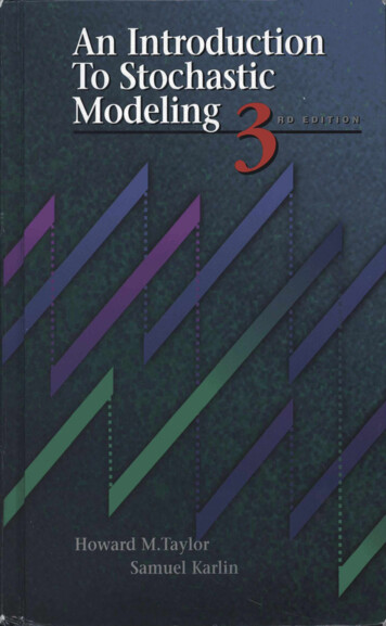
An IntroductionTo StochasticModelingHoward M.TaylorSamuel Karlin
An Introduction toStochastic ModelingThird Edition
An Introduction toStochastic ModelingThird EditionHoward M. TaylorStatistical ConsultantOnancock, Vi giniaSamuel KarlinDepartment of MathematicsStanford UniversityStanford, CaliforniaOAcademic PressSan DiegoLondonNew YorkSydneyBostonTokyoToronto
This book is printed on acid-free paper.Copyright 1998, 1994, 1984 by Academic PressAll rights reserved.No part of this publication may be reproduced ortransmitted in any form or by any means, electronicor mechanical, including photocopy, recording, orany information storage and retrieval system, withoutpermission in writing from the publisher.Permissions may be sought directly from Elsevier's Science and Technology Rights Department inOxford, UK. Phone: (44) 1865 843830, Fax: (44) 1865 853333, c-mail: permissions@elsevier.co.uk.You may also complete your request on-line via the Elsevier homepage: httpJ/www.elseviercom byselecting 'Customer Support' and then 'Obtaining Permissions'.ACADEMIC PRESSAn Imprint of Elsevier525 B St., Suite 1900, San Diego, California 92101-4495, USA1300 Boylston Street, Chestnut Hill, MA 02167, USAhttp://www.apnet.comAcademic Press Limited24-28 Oval Road, London NW 1 7DX, UKhttp://www.hbuk.co.uk/ap/Library of Congress Cataloging-in-Publication DataTaylor, Howard M.An introduction to stochastic modeling / Howard M. Taylor, SamuelKarlin. - 3rd ed.p.cm.Includes bibliographical references (p.ISBN-13: 978-0-12-684887-81. Stochastic processes.QA274.T35 1998003'.76--dc2l-) and index.ISBN-10: 0-12-684887-4I. Karlin, Samuel.ISBN-13: 978-0-12-684887-8ISBN-10: 0-12-684887-4PRINTED IN THE UNITED STATES OF AMERICA05060708 IP 987654II. Title.
ContentsPrefaceIIIIIIIntroductionix11. Stochastic Modeling2. Probability Review3. The Major Discrete Distributions4. Important Continuous Distributions5. Some Elementary Exercises6. Useful Functions, Integrals, and Sums624334353Conditional Probability and ConditionalExpectation571. The Discrete Case2. The Dice Game Craps3. Random Sums5764704. Conditioning on a Continuous Random Variable5. Martingales*7987Markov Chains: Introduction951. Definitions1952. Transition Probability Matrices of a Markov Chain1003. Some Markov Chain Models4. First Step Analysis5. Some Special Markov Chains1051161351516. Functionals of Random Walks and Success Runs*Stars indicate topics of a more advanced or specialized nature.
viContents7. Another Look at First Step Analysis*8. Branching Processes*9. Branching Processes and Generating Functions*169177184IV The Long Run Behavior of Markov Chains1991. Regular Transition Probability Matrices2. Examples1993. The Classification of States4. The Basic Limit Theorem of Markov Chains5. Reducible Markov Chains*V Poisson ProcessesVIVII2152342452582671. The Poisson Distribution and the Poisson Process2. The Law of Rare Events3. Distributions Associated with the Poisson Process4. The Uniform Distribution and Poisson Processes5. Spatial Poisson Processes6. Compound and Marked Poisson Processes267279290297Continuous Time Markov Chains3331. Pure Birth Processes2. Pure Death Processes3. Birth and Death Processes4. The Limiting Behavior of Birth and DeathProcesses5. Birth and Death Processes with Absorbing States6. Finite State Continuous Time Markov Chains7. A Poisson Process with a Markov Intensity*333345355Renewal Phenomena4191. Definition of a Renewal Process andRelated Concepts2. Some Examples of Renewal Processes3. The Poisson Process Viewed as a Renewal419426Process*Stars indicate topics of a more advanced or specialized nature.311318366379394408432
viiContents4. The Asymptotic Behavior of Renewal Processes4375. Generalizations and Variations on RenewalProcessesVIII4476. Discrete Renewal Theory*457Brownian Motion and Related Processes4731. Brownian Motion and Gaussian Processes4732. The Maximum Variable and the Reflection Principle 491IX3. Variations and Extensions4. Brownian Motion with Drift5. The Ornstein-Uhlenbeck Process*498508524Queueing Systems5411. Queueing Processes2. Poisson Arrivals, Exponential Service Times3. General Service Time Distributions4. Variations and Extensions5. Open Acyclic Queueing Networks6. General Open Networks541547558567581592Further Reading601Answers to Exercises603Index625*Stars indicate topics of a more advanced or specialized nature.
Preface to the First EditionStochastic processes are ways of quantifying the dynamic relationships ofsequences of random events. Stochastic models play an important role inelucidating many areas of the natural and engineering sciences. They canbe used to analyze the variability inherent in biological and medicalprocesses, to deal with uncertainties affecting managerial decisions andwith the complexities of psychological and social interactions, and to provide new perspectives, methodology, models, and intuition to aid in othermathematical and statistical studies.This book is intended as a beginning text in stochastic processes for students familiar with elementary probability calculus. Its aim is to bridgethe gap between basic probability know-how and an intermediate-levelcourse in stochastic processes-for example, A First Course in StochasticProcesses, by the present authors.The objectives of this book are three: (1) to introduce students to thestandard concepts and methods of stochastic modeling; (2) to illustrate therich diversity of applications of stochastic processes in the sciences; and(3) to provide exercises in the application of simple stochastic analysis toappropriate problems.The chapters are organized around several prototype classes of stochastic processes featuring Markov chains in discrete and continuoustime, Poisson processes and renewal theory, the evolution of branchingevents, and queueing models. After the concluding Chapter IX, we provide a list of books that incorporate more advanced discussions of severalof the models set forth in this text.
Preface to the Third EditionThe purposes, level, and style of this new edition conform to the tenets setforth in the original preface. We continue with our objective of introducing some theory and applications of stochastic processes to students hav-ing a solid foundation in calculus and in calculus-level probability, butwho are not conversant with the "epsilon-delta" definitions of mathematical analysis. We hope to entice students towards the deeper study ofmathematics that is prerequisite to further work in stochastic processes byshowing the myriad and interesting ways in which stochastic models canhelp us understand the real world.We have removed some topics and added others. We added a small section on martingales that includes an example suggesting the martingaleconcept as appropriate for modeling the prices of assets traded in a perfectmarket. A new chapter introduces the Brownian motion process and includes several applications of it and its variants in financial modeling. Inthis chapter the Black-Scholes formula for option pricing is evaluated andcompared with some reported prices of options. A Poisson process whoseintensity is itself a stochastic process is described in another new section.Some treatments have been updated. The law of rare events is presentedvia an inequality that measures the accuracy of a Poisson approximationfor the distribution of the sum of independent, not necessarily identicallydistributed, Bernoulli random variables. We have added the shot noisemodel and related it to a random sum.The text contains more than 250 exercises and 350 problems. Exercisesare elementary drills intended to promote active learning, to develop familiarity with concepts through use. They often simply involve the substitution of numbers into given formulas, or reasoning one or two stepsaway from a definition. They are the kinds of simple questions that we, as
instructors, hope that students would pose and answer for themselves asthey read a text. Answers to the exercises are given at the end of the bookso that students may gauge their understanding as they go along.Problems are more difficult. Some involve extensive algebraic or calculus manipulation. Many are "word problems" wherein the student isasked, in effect, to model some described scenario. As in formulating amodel, the first step in the solution of a word problem is often a sentenceof the form "Let x ." A manual containing the solutions to the problems is available from the publisher.A reasonable strategy on the part of the teacher might be to hold students responsible for all of the exercises, but to require submitted solutions only to selected problems. Every student should attempt a representative selection of the problems in order to develop his or her ability tocarry out stochastic modeling in his or her area of interest.A small number of problems are labeled "Computer Challenges." Thesecall for more than pencil and paper for their analyses, and either simulation, numerical exploration, or symbol manipulation may prove helpful.Computer Challenges are meant to be open-ended, intended to explorewhat constitutes an answer in today's world of computing power. Theymight be appropriate as part of an honors requirement.Because our focus is on stochastic modeling, in some instances we haveomitted a proof and contented ourselves with a precise statement of aresult and examples of its application. All such omitted proofs may befound in A First Course in Stochastic Processes, by the present authors.In this more advanced text, the ambitious student will also find additionalmaterial on martingales, Brownian motion, and renewal processes, andpresentations of several other classes of stochastic processes.
To the InstructorIf possible, we recommend having students skim the first two chapters, re-ferring as necessary to the probability review material, and starting thecourse with Chapter III, on Markov chains. A one quarter course adaptedto the junior-senior level could consist of a cursory (one-week) review ofChapters I and II, followed in order by Chapters III through VI. For interested students, Chapters VII, VIII, and IX discuss other currently activeareas of stochastic modeling. Starred sections contain material of a moreadvanced or specialized nature.AcknowledgmentsMany people helped to bring this text into being. We gratefully acknowl-edge the help of Anna Karlin, Shelley Stevens, Karen Larsen, andLaurieann Shoemaker. Chapter IX was enriched by a series of lectures onqueueing networks given by Ralph Disney at The Johns Hopkins University in 1982. Alan Karr, Ivan Johnstone, Luke Tierney, Bob Vanderbei,and others besides ourselves have taught from the text, and we have profited from their criticisms. Finally, we are grateful for improvements suggested by the several generations of students who have used the book overthe past few years and have given us their reactions and suggestions.
Chapter IIntroduction1.Stochastic ModelingA quantitative description of a natural phenomenon is called a mathematical model of that phenomenon. Examples abound, from the simpleequation S Zgt2 describing the distance S traveled in time t by a fallingobject starting at rest to a complex computer program that simulates abiological population or a large industrial system.In the final analysis, a model is judged using a single, quite pragmatic,factor, the model's usefulness. Some models are useful as detailed quantitative prescriptions of behavior, as for example, an inventory model thatis used to determine the optimal number of units to stock. Another modelin a different context may provide only general qualitative informationabout the relationships among and relative importance of several factorsinfluencing an event. Such a model is useful in an equally important butquite different way. Examples of diverse types of stochastic models arespread throughout this book.Such often mentioned attributes as realism, elegance, validity, andreproducibility are important in evaluating a model only insofar as theybear on that model's ultimate usefulness. For instance, it is both unrealistic and quite inelegant to view the sprawling city of Los Angeles as a geometrical point, a mathematical object of no size or dimension. Yet it isquite useful to do exactly that when using spherical geometry to derive aminimum-distance great circle air route from New York City, another"point."
2IIntroductionThere is no such thing as the best model for a given phenomenon. Thepragmatic criterion of usefulness often allows the existence of two ormore models for the same event, but serving distinct purposes. Considerlight. The wave form model, in which light is viewed as a continuous flow,is entirely adequate for designing eyeglass and telescope lenses. In con-trast, for understanding the impact of light on the retina of the eye, thephoton model, which views light as tiny discrete bundles of energy, ispreferred. Neither model supersedes the other; both are relevant anduseful.The word "stochastic" derives from the Greedto aim, toguess) and means "random" or "chance." The antonym is "sure," "deterministic," or "certain." A deterministic model predicts a single outcomefrom a given set of circumstances. A stochastic model predicts a set ofpossible outcomes weighted by their likelihoods, or probabilities. A coinflipped into the air will surely return to earth somewhere. Whether it landsheads or tails is random. For a "fair" coin we consider these alternativesequally likely and assign to each the probability 12.However, phenomena are not in and of themselves inherently stochas-tic or deterministic. Rather, to model a phenomenon as stochastic or deterministic is the choice of the observer. The choice depends on the observer's purpose; the criterion for judging the choice is usefulness. Mostoften the proper choice is quite clear, but controversial situations do arise.If the coin once fallen is quickly covered by a book so that the outcome"heads" or "tails" remains unknown, two participants may still usefullyemploy probability concepts to evaluate what is a fair bet between them;that is, they may usefully view the coin as random, even though most people would consider the outcome now to be fixed or deterministic. As a lessmundane example of the converse situation, changes in the level of a largepopulation are often usefully modeled deterministically, in spite of thegeneral agreement among observers that many chance events contributeto their fluctuations.Scientific modeling has three components: (i) a natural phenomenonunder study, (ii) a logical system for deducing implications about the phenomenon, and (iii) a connection linking the elements of the natural systemunder study to the logical system used to model it. If we think of thesethree components in terms of the great-circle air route problem, the natural system is the earth with airports at Los Angeles and New York; thelogical system is the mathematical subject of spherical geometry; and the
1.Stochastic Modeling3two are connected by viewing the airports in the physical system as pointsin the logical system.The modern approach to stochastic modeling is in a similar spirit. Nature does not dictate a unique definition of "probability," in the same waythat there is no nature-imposed definition of "point" in geometry. "Probability" and "point" are terms in pure mathematics, defined only throughthe properties invested in them by their respective sets of axioms. (SeeSection 2.8 for a review of axiomatic probability theory.) There are, however, three general principles that are often useful in relating or connecting the abstract elements of mathematical probability theory to a real ornatural phenomenon that is to be modeled. These are (i) the principle ofequally likely outcomes, (ii) the principle of long run relative frequency,and (iii) the principle of odds making or subjective probabilities. Historically, these three concepts arose out of largely unsuccessful attempts todefine probability in terms of physical experiences. Today, they are relevant as guidelines for the assignment of probability values in a model, andfor the interpretation of the conclusions of a model in terms of the phenomenon under study.We illustrate the distinctions between these principles with a long experiment. We will pretend that we are part of a group of people who decide to toss a coin and observe the event that the coin will fall heads up.This event is denoted by H, and the event of tails, by T.Initially, everyone in the group agrees that Pr{H} ;. When asked why,people give two reasons: Upon checking the coin construction, they believe that the two possible outcomes, heads and tails, are equally likely;and extrapolating from past experience, they also believe that if the coinis tossed many times, the fraction of times that heads is observed will beclose to one-half.The equally likely interpretation of probability surfaced in the works ofLaplace in 1812, where the attempt was made to define the probability ofan event A as the ratio of the total number of ways that A could occur tothe total number of possible outcomes of the experiment. The equallylikely approach is often used today to assign probabilities that reflect somenotion of a total lack of knowledge about the outcome of a chance phenomenon. The principle requires judicious application if it is to be useful,however. In our coin tossing experiment, for instance, merely introducingthe possibility that the coin could land on its edge (E) instantly results inPr(H) Pr{T} Pr{E} ;.
4IIntroductionThe next principle, the long run relative frequency interpretation ofprobability, is a basic building block in modern stochastic modeling, madeprecise and justified within the axiomatic structure by the law of largenumbers. This law asserts that the relative fraction of times in which anevent occurs in a sequence of independent similar experiments approaches, in the limit, the probability of the occurrence of the event on anysingle trial.The principle is not relevant in all situations, however. When the surgeon tells a patient that he has an 80-20 chance of survival, the surgeonmeans, most likely, that 80 percent of similar patients facing similarsurgery will survive it. The patient at hand is not concerned with the longrun, but in vivid contrast, is vitally concerned only in the outcome of his,the next, trial.Returning to the group experiment, we will suppose next that the coin isflipped into the air and, upon landing, is quickly covered so that no one cansee the outcome. What is Pr{H} now? Several in the group argue that theoutcome of the coin is no longer random, that Pr{H} is either 0 or 1, andthat although we don't know which it is, probability theory does not apply.Others articulate a different view, that the distinction between "random" and "lack of knowledge" is fuzzy, at best, and that a person with asufficiently large computer and sufficient information about such factorsas the energy, velocity, and direction used in tossing the coin could havepredicted the outcome, heads or tails, with certainty before the toss.Therefore, even before the coin was flipped, the problem was a lack ofknowledge and not some inherent randomness in the experiment.In a related approach, several people in the group are willing to bet witheach other, at even odds, on the outcome of the toss. That is, they are willing to use the calculus of probability to determine what is a fair bet, without considering whether the event under study is random or not. The usefulness criterion for judging a model has appeared.While the rest of the mob were debating "random" versus "lack ofknowledge," one member, Karen, looked at the coin. Her probability forheads is now different from that of everyone else. Keeping the coin covered, she announces the outcome "Tails," whereupon everyone mentallyassigns the value Pr{H} 0. But then her companion, Mary, speaks upand says that Karen has a history of prevarication.The last scenario explains why there are horse races; different peopleassign different probabilities to the same event. For this reason, probabil-
1.Stochastic Modeling5ities used in odds making are often called subjective probabilities. Then,odds making forms the third principle for assigning probability values inmodels and for interpreting them in the real world.The modern approach to stochastic modeling is to divorce the definitionof probability from any particular type of application. Probability theoryis an axiomatic structure (see Section 2.8), a part of pure mathematics. Itsuse in modeling stochastic phenomena is part of the broader realm of science and parallels the use of other branches of mathematics in modelingdeterministic phenomena.To be useful, a stochastic model must reflect all those aspects of thephenomenon under study that are relevant to the question at hand. In addition, the model must be amenable to calculation and must allow the deduction of important predictions or implications about the phenomenon.1.1.Stochastic ProcessesA stochastic process is a family of random variables X where t is a parameter running over a suitable index set T. (Where convenient, we willwrite X(t) instead of X,.) In a common situation, the index t correspondsto discrete units of time, and the index set is T {0, 1, 2, . . .}. In thiscase, X, might represent the outcomes at successive tosses of a coin, repeated responses of a subject in a learning experiment, or successive ob-servations of some characteristics of a certain population. Stochasticprocesses for which T [0, c) are particularly important in applications.Here t often represents time, but different situations also frequently arise.For example, t may represent distance from an arbitrary origin, and X, maycount the number of defects in the interval (0, t] along a thread, or thenumber of cars in the interval (0, t] along a highway.Stochastic processes are distinguished by their state space, or the rangeof possible values for the random variables X by their index set T, and bythe dependence relations among the random variables X,. The most widelyused classes of stochastic processes are systematically and thoroughlypresented for study in the following chapters, along with the mathematical techniques for calculation and analysis that are most useful with theseprocesses. The use of these processes as models is taught by example.Sample applications from many and diverse areas of interest are an integral part of the exposition.
62.IIntroductionProbability Review*This section summarizes the necessary background material and establishes the book's terminology and notation. It also illustrates the level ofthe exposition in the following chapters. Readers who find the major partof this section's material to be familiar and easily understood should haveno difficulty with what follows. Others might wish to review their probability background before continuing.In this section statements frequently are made without proof. Thereader desiring justification should consult any elementary probabilitytext as the need arises.2.1.Events and ProbabilitiesThe reader is assumed to be familiar with the intuitive concept of an event.(Events are defined rigorously in Section 2.8, which reviews the axiomaticstructure of probability theory.)Let A and B be events. The event that at least one of A or B occurs iscalled the union of A and B and is written A U B; the event that both occuris called the intersection of A and B and is written A fl B, or simply AB.This notation extends to finite and countable sequences of events. Givenevents A A2, . , the event that at least one occurs is written A, U A, U U i A;, the event that all occur is written A, fl A, fl f1; , A;.The probability of an event A is written Pr{A }. The certain event, denoted by (1, always occurs, and Pr{ Cl } 1. The impossible event, denoted by 0, never occurs, and Pr{O} 0. It is always the case that 0 sPr(A) : 1 for any event A.Events A, B are said to be disjoint if A fl B 0; that is, if A and Bcannot both occur. For disjoint events A, B we have the addition lawPr{A U B) Pr(A) Pr{B}. A stronger form of the addition law is asfollows: Let A,, A,, . . . be events with A; and A; disjoint whenever i 0 j.Then Pr(U , A; ) Ex , Pr{A;}. The addition law leads directly to the law* Many readers will prefer to omit this review and move directly to Chapter III, onMarkov chains. They can then refer to the background material that is summarized in theremainder of this chapter and in Chapter II only as needed.
2.Probability Review7be disjoint events for which fl A, U A,U . Equivalently, exactly one of the events A A,. . . will occur. The lawof total probability asserts that Pr{B} 7-; , Pr(B fl A;} for any event B.of total probability: Let A,, A,, . .The law enables the calculation of the probability of an event B fromthe sometimes more easily determined probabilities Pr{B fl A;}, where i 1, 2, . Judicious choice of the events A; is prerequisite to the profitable application of the law.Events A and B are said to be independent if Pr{A fl B) Pr{A} XPr{B}. Events A,, A,, . are independent ifPr{A;1 fl A;, fl . fl A; } Pr(A;d Pr{A;,} . Pr{A; }for every finite set of distinct indices i i,, .2.2., i,,.Random VariablesAn old-fashioned but very useful and highly intuitive definition describesa random variable as a variable that takes on its values by chance. In Section 2.8, we sketch the modern axiomatic structure for probability theoryand random variables. The older definition just given serves quite adequately, however, in virtually all instances of stochastic modeling. Indeed,this older definition was the only approach available for well over a century of meaningful progress in probability theory and stochasticprocesses.Most of the time we adhere to the convention of using capital letterssuch as X, Y, Z to denote random variables, and lowercase letters such asx, y, z for real numbers. The expression (X:5 x) is the event that the random variable X assumes a value that is less than or equal to the real number x. This event may or may not occur, depending on the outcome of theexperiment or phenomenon that determines the value for the random variable X. The probability that the event occurs is written Pr{X - x). Allowing x to vary, this probability defines a functionF(x) Pr{Xx},-oo x o,called the distribution function of the random variable X. Where severalrandom variables appear in the same context, we may choose to distinguish their distribution functions with subscripts, writing, for example,FX(6) Pr(X --- ) and F,.(6) Pr{ Y6}, defining the distribution
8IIntroductionfunctions of the random variables X and Y, respectively, as functions ofthe real variable 6.The distribution function contains all the information available about arandom variable before its value is determined by experiment. We have,for instance, Pr{X a} 1 - F(a), Pr{a X b} F(b) - F(a), andPr{X x} F(x) - lim.10 F(x - e) F(x) - F(x -).A random variable X is called discrete if there is a finite or denumerableset of distinct values x,, x2, . such that a, Pr{X x; } 0 for i 1, 2,. and Y a; 1. The functionp(x,) px(x;) a;for i 1, 2,.(2.1)is called the probability mass function for the random variable X and is related to the distribution function viap(x;) F(x,) - F(x; -) and F(x)p(x;).xi xThe distribution function for a discrete random variable is a step function,which increases only in jumps, the size of the jump at x; being p(x;).If Pr{X x} 0 for every value of x, then the random variable Xis called continuous and its distribution function F(x) is a continuousfunction of x. If there is a nonnegative function f(x) fx(x) defined for-- x - such thatnPr{a X b} Jf(x)dxfor -oo a b co,(2.2)athen f(x) is called the probability density function for the random variableX. If X has a probability density function f(x), then X is continuous andF(x)f(6) de,-o- x -.If F(x) is differentiable in x, then X has a probability density functiongiven byf(x) d F(x) F'(x),-00 x 00.(2.3)In differential form, (2.3) leads to the informal statementPr { x X x dx } F(x dx) - F(x) dF(x) f (x) dx. (2.4)
2.Probability Review9We consider (2.4) to be a shorthand version of the more precise statementPr{x X -x Ax} f(x)L x o(Ox),Ax 10,(2.5)where o(Ax) is a generic remainder term of order less than Ox as Ax 10.That is, o(1x) represents any term for which lima,10 o(Ax)/Ax 0. By thefundamental theorem of calculus, equation (2.5) is valid whenever theprobability density function is continuous at x.While examples are known of continuous random variables that do notpossess probability density functions, they do not arise in stochastic modelsof common natural phenomena.2.3.Moments and Expected ValuesIf X is a discrete random variable, then its mth moment is given byE[X",]x' Pr(X x;},(2.6)[where the x; are specified in (2.1)] provided that the infinite sum converges absolutely. Where the infinite sum diverges, the moment is said notto exist. If X is a continuous random variable with probability densityfunctionf(x), then its mth moment is given byE[X"] J x";f(x) dx,(2.7)provided that this integral converges absolutely.The first moment, corresponding to m 1, is commonly called themean or expected value of X and written m, or µX. The mth central moment of X is defined as the mth moment of the random variable X - tt,provided that p exists. The first central moment is zero. The second central moment is called the variance of X and written oX or Var[X]. We havethe equivalent formulas Var[X] E[(X - µ)2] E[X2] - Al.The median of a random variable X is any value v with the property thatPr{X ? v) ?andPr{X :s v} ? Z.If X is a random variable and g is a function, then Y g(X) is also a
10IIntroductionrandom variable. If X is
Preface to the Third Edition The purposes, level, and style of this new edition conform to the tenets set forth in the original preface. We continue with our objective of introduc-ing some theory and applications of stochastic processes to students hav-ing a solid foun
