WIXLIB

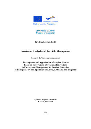
OutlineAsset ReturnsMarkowitz’s Portfolio TheoryCAPMMultifactor Pricing ModelsResampling MethodsThe CAPMOne Fund TheoremThere is a single fund M of risky assets such that any efficient portfoliocan be constructed as a linear combination of the fund M and therisk-free asset.When short selling is allowed, the minimum-variance portfolio (MVP)with the expected return µ can be computed by solving the optimizationproblemmin wT Σw subject to wT µ (1 wT 1)rf µ .wThe problem has an explicit solution for w when Σ is nonsingular:weff (µ rf )Σ 1 (µ rf 1) 1T(µ rf 1) Σ (µ rf 1) Σ 1 (µ rf 1)/[1T Σ 1 (µ rf 1)](The fund)Haipeng XingSUNY Stony BrookBasic investment models and their statistical analysisOutlineAsset ReturnsMarkowitz’s Portfolio TheoryCAPMMultifactor Pricing ModelsResampling MethodsSharpe ratio and the capital market lineFor a portfolio whose return has mean µ and variance σ 2 , its Sharperatio is (µ rf )/σ, which is the expected excess return per unit ofrisk.The straight line joining (0, rf ) and the tangent point M in Figure5, which is the efficient frontier in the presence of a risk-free asset, iscalled the capital market line and given byµ rf µM rfσ;σMi.e., the Sharpe ratio of any efficient portfolio is the same as that ofthe market portfolio.Haipeng XingBasic investment models and their statistical analysisSUNY Stony Brook

OutlineAsset ReturnsMarkowitz’s Portfolio TheoryCAPMMultifactor Pricing ModelsResampling MethodsBeta and the security market lineThe beta, denoted by βi , of risky asset i that has return ri is defined2by βi Cov(ri , rM )/σM. The CAPM relates the expected excessreturn (also called the risk premium) µi rf of asset i to its betaviaµi rf βi (µM rf ),which is referred to as the security market line.The above linear relationship can be rewritten asri rf βi (rM rf ) &i ,in which E(&i ) 0 and Cov(&i , rM ) 0, it follows that2σi2 βi2 σM Var(&i ),decomposing the variance σi2 of the ith asset return as a sum of the2systematic risk βi2 σM, which that is associated with the market, andthe idiosyncratic risk, which is unique to the asset and uncorrelatedwith market movements.Haipeng XingSUNY Stony BrookBasic investment models and their statistical analysisOutlineAsset ReturnsMarkowitz’s Portfolio TheoryCAPMMultifactor Pricing ModelsResampling MethodsInvestment implicationsUsing β as a measure of risk, the Treynor index is defined by(µ rf )/β.The Jensen index is the α in the generalization of CAPM toµ rf α β(µM rf ). An investment with a positive α isconsidered to perform better than the market.Jensen (1968) perform an empirical study using the regression modelµ rf α β(µM rf ) &. His findings support the efficientmarket hypothesis, according to which it is not possible tooutperform the market portfolio in an efficient market.Haipeng XingBasic investment models and their statistical analysisSUNY Stony Brook

OutlineAsset ReturnsMarkowitz’s Portfolio TheoryCAPMMultifactor Pricing ModelsResampling MethodsEstimation and testingLet yt be a q 1 vector of excess returns on q assets and let xt be theexcess return on the market portfolio (or, more precisely, its proxy) attime t. The CAPM can be associated with the null hypothesisH0 : α 0 in the regression modelyt α xt β #t ,1 t n,(1)where E(#t ) 0, Cov(#t ) V, and E(xt #t ) 0.)n)nLetting x̄ n 1 t 1 xt and ȳ n 1 t 1 yt , the ordinary leastsquares (OLS) estimates of α and β are given by)n(xt x̄)yt00 )t 10 ȳ x̄β.,αβn2(x x̄)t 1 tHaipeng Xing(2)SUNY Stony BrookBasic investment models and their statistical analysisOutlineAsset ReturnsMarkowitz’s Portfolio TheoryCAPMMultifactor Pricing ModelsResampling MethodsEstimation and testingThe maximum likelihood estimate of V is0 nV 1n"t 10 t )(yt α0 t )T .0 βx0 βx(yt α(3)The properties of OLS can be used to establish the asymptotic normality0 and α,0 yielding the approximationsof β%&% %& &20V1x̄0 N β, )n0 ,0 N α,,αβV )n22(x x̄)(x x̄)nttt 1t 1from which approximate confidence regions for β and α can beconstructed.Haipeng XingBasic investment models and their statistical analysisSUNY Stony Brook

OutlineAsset ReturnsMarkowitz’s Portfolio TheoryCAPMMultifactor Pricing ModelsResampling MethodsEstimation and testingWhen #t are i.i.d. normal and are independent of the market excess0 and V0 are the maximum likelihood estimates of α, β,0 , β,returns xt , α0 V)0 given0 β,and V. Furthermore, the conditional distribution of (α,(x1 , . . . , xn ) are expressed as( (' '1x̄20 N α, )nV ,(4)α2n(x x̄)tt 1'(V0 N β, )n0 Wq (V, n 2),β, nV2(x x̄)t 1 t0 Moreover, we can show that, under H0 ,0 independent of (α,0 β).with V.*'n q 1(x̄2T 0 1)0 V α0 Fq,n q 1 . (5)α1 1 n2qnt 1 (xt x̄)Note that (5) still holds approximately without the normality assumptionwhen n q 1 is moderate or large.Haipeng XingSUNY Stony BrookBasic investment models and their statistical analysisOutlineAsset ReturnsMarkowitz’s Portfolio TheoryCAPMMultifactor Pricing ModelsResampling MethodsAn illustrative exampleWe illustrate the statistical analysis of CAPM with the monthly returnsdata of the six stocks in the previous section using the Dow JonesIndustrial Average index as the market portfolio M and the 3-month U.S.Treasury bill as the risk-free asset. These data are used to estimatequantities in Table 2.Table 2: Performance of six stocks from August 2000 to October 2005.α 103p-value β2 104β 2 σM2σ! 104Sharpe 102Treynor 103AXPCITIXOMGMINTELPFE0.870.721.235.773.50 5.49 1.350.810.761.205.484.18 5.36 1.382.230.400.521.044.225.052.22 2.410.591.447.9112.0 12.1 3.74 4.310.522.2819.826.7 13.2 3.96 5.210.060.460.804.64 26.4 13.4 refers to the p-value of the t-test of H0 : αi 0.Haipeng XingBasic investment models and their statistical analysisSUNY Stony Brook

OutlineAsset ReturnsMarkowitz’s Portfolio TheoryCAPMMultifactor Pricing ModelsResampling MethodsEmpirical literature on the CAPMSince the development of CAPM in the 1960s, a large body of literaturehas evolved on empirical evidence for or against the model. The earlyevidence was largely positive, but in the late 1970s, less favorableevidence began to appear.Basu (1977) reported the “price–earnings-ratio effect”: Firms withlow price–earnings ratios have higher average returns, and firms withhigh price–earnings ratios have lower average returns than the valuesimplied by CAPM.Banz (1981) noted the “size effect,” that firms with low marketcapitalizations have higher average returns than under CAPM.Haipeng XingSUNY Stony BrookBasic investment models and their statistical analysisOutlineAsset ReturnsMarkowitz’s Portfolio TheoryCAPMMultifactor Pricing ModelsResampling MethodsEmpirical literature on the CAPMFama and French (1992, 1993) have found that beta cannot explainthe difference in returns between portfolios formed on the basis ofthe ratio of book value to market value of equity.Jegadesh and Titman (1995) have noted that a portfolio formed bybuying stocks whose values have declined and selling stocks whosevalues have risen has a higher average return than predicted byCAPM.Remark 3The empirical study for or against CAPM might involves the issues ofdata snooping, selection bias, and proxy bias.Haipeng XingBasic investment models and their statistical analysisSUNY Stony Brook

OutlineAsset ReturnsMarkowitz’s Portfolio TheoryCAPMMultifactor Pricing ModelsResampling MethodsArbitrage pricing theory (APT)Multifactor pricing models generalize CAPM by embedding it in aregression model of the formri αi β Ti f &i ,i 1, · · · , p,(6)in which the ri is the return on the ith asset, αi and β i areunknown regression parameters, f (f1 , . . . , fk )T is a regressionvector of factors, and &i is an unobserved random disturbance thathas mean 0 and is uncorrelated with f .Ross (1976) introduced the APT which allows multiple risk factorsfor asset returns. Unlike the CAPM, APT does not requireidentification of the market portfolio and relates the expected returnµi of the ith asset to the risk-free return, or to a more generalparameter λ0 without assuming the existence of a risk-free asset,and to a k 1 vector λ of risk premiums:µi λ0 β Ti λ,i 1, . . . , p.Haipeng Xing(7)SUNY Stony BrookBasic investment models and their statistical analysisOutlineAsset ReturnsMarkowitz’s Portfolio TheoryCAPMMultifactor Pricing ModelsResampling MethodsArbitrage pricing theory (APT)While APT provides an economic theory underlying multifactormodels of asset returns, the theory does not identify the factors.Approaches to the choice of factors can be broadly classified aseconomic and statistical.The economic approach specifies (i) macroeconomic and financialmarket variables that are thought to capture the systematic risks ofthe economy or (ii) characteristics of firms that are likely to explaindifferential sensitivity to the systematic risks, forming factors fromportfolios of stocks based on the characteristics.The statistical approach uses factor analysis or PCA (principalcomponent analysis) to estimate the parameters of model (6) from aset of observed asset returns.Haipeng XingBasic investment models and their statistical analysisSUNY Stony Brook

OutlineAsset ReturnsMarkowitz’s Portfolio TheoryCAPMMultifactor Pricing ModelsResampling MethodsFactor analysisLetting r (r1 , . . . , rp )T , α (α1 , . . . , αp )T , # (&1 , . . . , &p )T , and Bto be the p k matrix whose ith row vector is βTi , we can rewrite themultifactor pricing model (6) as r α Bf # with E# Ef 0 andE(f #T ) 0. Note that the regressor f is unobservable.Let rt , t 1, . . . , n, be independent observations from the model so thatrt α Bf t #t and E#t Eft 0, E(ft #Tt ) 0, Cov(ft ) Ω, andCov(#t ) V. ThenE(rt ) α,Cov(rt ) BΩBT V.(8)The decomposition of the covariance matrix Σ of rt in (8) is the essenceof factor analysis, which separates variability into a systematic part dueto the variability of certain unobserved factors, represented by BΩBT ,and an error (idiosyncratic) part, represented by V.Haipeng XingSUNY Stony BrookBasic investment models and their statistical analysisOutlineAsset ReturnsMarkowitz’s Portfolio TheoryCAPMMultifactor Pricing ModelsResampling MethodsThe factor analysis — IdentifiabilityIn standard factor analysis, V is assumed to be diagonal; i.e.,V diag(v1 , . . . , vp ). Since B and Ω are not uniquely determined byΣ BΩBT V, the orthogonal factor model assumes that Ω I sothat B is unique up to an orthogonal transformation andr α Bβ # with Cov(f ) Ω yieldsCov(r, f ) E{(r α)f T } BΩ B,Var(ri ) k"b2ij Var(&i ),1 i p,(9)(10)j 1Cov(ri , rj ) k"bil bjl ,1 i, j p.(11)l 1Haipeng XingBasic investment models and their statistical analysisSUNY Stony Brook

OutlineAsset ReturnsMarkowitz’s Portfolio TheoryCAPMMultifactor Pricing ModelsResampling MethodsThe factor analysis — MLEAssuming the observed rt to be independent N (α, Σ), the likelihoodfunction is12n"1L(α, Σ) (2π) pn/2 (det Σ) n/2 exp (rt α)T Σ 1 (rt α) ,2 t 1with Σ constrained to be of the form Σ BBT ) diag(v1 , . . . , vp ), in0 of α is r̄ : n 1 nt 1 rt , and we canwhich B is p k. The MLE αn log det(Σ) 21 tr(WΣ 1 ) over Σ of the form above,maximize 21)nwhere W t 1 (rt r̄)(rt r̄)T . Iterative algorithms can be used to0 and therefore also B0 and v01 , . . . , 0find the maximizer Σvp .Haipeng XingSUNY Stony BrookBasic investment models and their statistical analysisOutlineAsset ReturnsMarkowitz’s Portfolio TheoryCAPMMultifactor Pricing ModelsResampling MethodsThe factor analysis — factor rotation0 are called factor loadings.In factor analysis, the entries of the matrix B0 is unique only up to orthogonal transformations, the usualSince B0 by a suitably chosen orthogonal matrix Q,practice is to multiply Bcalled a factor rotation, so that the factor loadings have a simple0 BQ,0interpretable structure. Letting Ba popular choice of Q is thatwhich maximizes the varimax criterion# p% p&2 k."""0b 4 0b 2pC p 1ijj 1 k"j 1i 1iji 1 ,Var squared loadings of the jth factor .Haipeng XingBasic investment models and their statistical analysisSUNY Stony Brook

OutlineAsset ReturnsMarkowitz’s Portfolio TheoryCAPMMultifactor Pricing ModelsResampling MethodsThe factor analysis — factor scoresSince the values of the factors ft , 1 t n, are unobserved, it is oftenof interest to impute these values, called factor scores, for modeldiagnostics. From the model r α Bf # with Cov(#) V, thegeneralized least squares estimate of f when B, V, and α are known is0f (BT V 1 B) 1 BT V 1 (rt α).Bartlett (1937) therefore suggested estimating ft by00TV0 1 B)0 1 B0TV0 1 (rt r̄).ft (BHaipeng Xing(12)SUNY Stony BrookBasic investment models and their statistical analysisOutlineAsset ReturnsMarkowitz’s Portfolio TheoryCAPMMultifactor Pricing ModelsResampling MethodsThe factor analysis — the number of factorsThe theory underlying multifactor pricing models and factor analysisassumes that the number k of factors has been specified and doesnot indicate how to specify it.When the rt are independent N (α, Σ), we may consider a formalhypothesis testing that the k-factor model indeed holds. The nullhypothesis H0 is that Σ BBT V with V diagonal and B beingp k.The generalized likelihood ratio statistic that tests the H0 againstunconstrained Σ is of the form* , ,T0000 ,(13)Λ n log det BB V log det Σ0 n 1 )n (rt r̄)(rt r̄)T is the unconstrained MLE ofwhere Σt 1Σ.Haipeng XingBasic investment models and their statistical analysisSUNY Stony Brook

OutlineAsset ReturnsMarkowitz’s Portfolio TheoryCAPMMultifactor Pricing ModelsResampling MethodsThe factor analysis — the number of factorsUnder H0 , Λ is approximately χ2 with*- 13411(p k)2 p kp(p 1) p(k 1) k(k 1) 222degrees of freedom.Bartlett (1954) has shown that the χ2 approximation to thedistribution of (13) can be improved by replacing n in (13) byn 1 (2p 4k 5)/6, which is often used in empirical studies.Haipeng XingSUNY Stony BrookBasic investment models and their statistical analysisOutlineAsset ReturnsMarkowitz’s Portfolio TheoryCAPMMultifactor Pricing ModelsResampling MethodsThe PCA approachThe fundamental decomposition Σ λ1 a1 aT1 · · · λp ap aTp inPCA (see Section 2.2.2) can be used to decompose Σ intoΣ BBT V. Here λ1 · · · λp are the ordered eigenvalues ofΣ, ai is the unit eigenvector associated with λi , and55B ( λ1 a1 , . . . , λk ak ),V p"λl al aTl .(14)l k 1PCA is particularly useful when most eigenvalues of Σ are small incomparison with the k largest ones, so that k principal componentsof rt r̄ account for a large proportion of the overall variance. Inthis case, we can use PCA to determine k.Haipeng XingBasic investment models and their statistical analysisSUNY Stony Brook

OutlineAsset ReturnsMarkowitz’s Portfolio TheoryCAPMMultifactor Pricing ModelsResampling MethodsThe Fama-French three-factor modelFama and French (1993, 1996) propose a three-factor model whichhas the formE(ri ) rf αi β Ti (rM rf , rS rL , rH rL )T .The factor rM rf is the only factor in the CAPM. The factorrS rL captures the risk factor in returns related to size. Here“small” and “large” refer to the market value of equity. The factorrH rL , which captures the risk factor in returns related to thebook-to-market equity.Fama and French (1992, 1993) argue that their three-factor modelremoves most of the pricing anomalies with CAPM. Because thefactors in the Fama-French model are specified, one can use standardregression analysis to test the model and estimate its parameters.Haipeng XingSUNY Stony BrookBasic investment models and their statistical analysisOutlineAsset ReturnsMarkowitz’s Portfolio TheoryCAPMMultifactor Pricing ModelsResampling MethodsBootstrap estimate of the CAPMWe illustrate how bootstrap resampling can be applied to estimatethe CAPM in Table 2 based on the monthly excess log returns of sixstocks from August 2000 to October 2005. The α and β in thetable are estimated by applying OLS to the regression modelri rf αi βi (rM rf ) &i , in which the market portfolio M istaken to be the Dow Jones Industrial Average index and rf is theannualized rate of the 3-month U.S. Treasury bill.Let xt rM,t rf,t and yi,t ri,t rf,t . We draw B 500 bootstrap samples {(x t , yi,t), 1 t n 63} from the observedsample {(xt , yi,t ), 1 t n 63} and compute the OLS estimates α0 i and β0i for the regression model yi,t α i βi x t & t . We thenreport in Table 3 the average values of α0 i , β0i , Sharpe index andTreynor index of the B bootstrap samples, and their standarddeviations (given in parentheses).Haipeng XingBasic investment models and their statistical analysisSUNY Stony Brook

OutlineAsset ReturnsMarkowitz’s Portfolio TheoryCAPMMultifactor Pricing ModelsResampling MethodsBootstrap estimate of the CAPMTable 3: Bootstrapping CAPM.α 103βSharpe 102Treynor 103AXPCITI1.00 (0.28)0.84 (0.32)1.23 (0.02)1.20 (0.02) 4.51 (1.61) 5.16 (1.60) 1.14 (0.40) 1.36 (0.41)XOMGM2.24 (0.33) 1.99 (0.58)0.53 (0.02)1.44 (0.04)4.69 (1.59) 12.2 (1.65)2.27 (0.75) 4.02 (0.57)IntelPfizer 4.33 (0.74) 5.23 (0.33)2.29 (0.05)0.45 (0.02) 13.0 (1.44) 26.2 (1.62) 3.95 (0.44) 13.5 (4.05)Haipeng XingSUNY Stony BrookBasic investment models and their statistical analysisOutlineAsset ReturnsMarkowitz’s Portfolio TheoryCAPMMultifactor Pricing ModelsResampling MethodsMichaud’s resampled efficient frontierAs pointed out before, the estimated (“plug-in”) efficient frontier0 differs from0 and covariance matrix Σbased on the sample mean µthe true efficient frontier. Frankfurter, Phillips, and Seagle (1971)and Jobson and Korkie (1980) have found that portfolios thusconstructed may per

Outline Asset Returns Markowitz’s Portfolio Theory CAPM Multifactor Pricing Models Resampling Methods Statistical models for asset prices and returns A commonly used model for risky asset prices P t is geometric Brownian motion (GBM), with volatility σ and instantaneous rate of