WIXLIB

Theoretical Economics Letters, 2018, 8, 2095-2102http://www.scirp.org/journal/telISSN Online: 2162-2086ISSN Print: 2162-2078Solving Basic Inventory Models Using ExcelSarbjit SinghInstitute of Management Technology, Nagpur, IndiaHow to cite this paper: Singh, S. (2018)Solving Basic Inventory Models Using Excel.Theoretical Economics Letters, 8, eceived: May 31, 2018Accepted: August 3, 2018Published: August 6, 2018Copyright 2018 by author andScientific Research Publishing Inc.This work is licensed under the CreativeCommons Attribution InternationalLicense (CC BY en AccessAbstractIn this note, I have introduced a simple way to solve the four basic inventorymodels using Microsoft excel. This note can be used in courses like economics, operations management, operations research, supply chain management.This note can be used in teaching basic inventory models to avoid the lengthymanual calculation involved in solving them. It can also be used as an interesting example for an advanced class in Excel. The user just needs to enter thedata in the white cells and all the results are automatically calculated. Werecommend showing students how to first solve the models by hand (notnecessarily the example problem), so that they understand the procedure, andthen show them how to do it using Excel. The four models considered hereare EOQ model, Basic production model, Discount Model and ShortageModel. Using the excel managers would be able to compare the various scenarios provided by the organization. They would find it very convenient touse these models.KeywordsEOQ Model, Production Model, Shortage Model, Discount Model1. IntroductionInventory management involves decisions about the level of inventory, organization should keep to get the maximum profit. Inventory has been defined asidle resources that possess economic value by Monks [1]. To meet demand ontime, companies often keep on hand stock that is awaiting sale. The purpose ofinventory management is minimizing the cost associated with keeping inventoryand meeting customer expectations. The two basic questions of inventory management are: 1) When should an order be placed for an Item? 2) How largeshould each order be?Economic order quantity model was first developed by Ford Harris [2], but R.H. Wilson [3] applied it extensively, that is, why this is also known as Harris andDOI: 10.4236/tel.2018.811137 Aug. 6, 20182095Theoretical Economics Letters

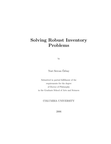
S. SinghWilson model. There is mention of economic order quantity as minimal quantity cost in book purchasing and storing by Ralph Currier Davis [4]. The aim isto decide an optimal ordering quantity, Q, which minimizes the total cost ofan inventory system when the demand occurs at a constant rate. Hadley andWhitin [5] have analyzed economic order quantity model and studied its applications in practical scenarios. James M. Cargal [6] also worked on the EOQformula and he also tried to find why large number of organizations are still using EOQ formula even it has some unrealistic assumptions. David Piasecki [7]formulated how to optimize cost using EOQ and also deal with conflict betweenJIT and EOQ.This article deals with the solution of some elementary inventory models. Thenote deals with the basic EOQ and its extensions. In this note I have introducedthe basic models and also given their excel programs so by using this programs,students can solve the inventory related issues by applying the various elementary models. The programs developed are user friendly and various inventoryrelated problems can be solved using them.2. The Advantages of Having Large InventoryEarlier most of the organizations used to keep large inventories. As it has lots ofbenefits, one of the main reasons was unhampered production. Also buyingitems in bulk help organizations to get better discounts. Even transportation costreduces if items are bought in bulk. The customer satisfaction increases as services would be smooth and faster. Some time it also helps in case of items whichare seasonal items, hence helps in price speculations.3. The Disadvantages of Having a Large InventoryLike every coin has two sides, keeping large inventory also has numerous disadvantages. To keep a large inventory, a lot of money is invested which can be usedfor some other purpose. To keep a large inventory, a lot of money is spending onwarehouse rent, accounting and insurance. Also, many items start deterioratingafter some time. Some of the items become obsolete after some fixed time.4. Economic Order Quantity ModelThe EOQ model is the elementary model and has the following assumptions.The demand is deterministic and constant over time. Shortages are not allowed,the Lead time is either zero or constant. Order quantity is instantaneous (Figure1).S—Cost of placing order; D—Annual demand; H—Annual per-unit carryingcost; Q—Order quantity; Annual Ordering Cost S * D/Q; Annual CarryingCost H * Q/2; Total Inventory Cost S * D/Q H * D/2; Number of Orders D/Q; Average Inventory Q/2.CASE I—Shamole India Ltd. is a supplier of filter to Monu Tractors. It supplies fifty thousand tractors to Monu Tractors annually. At Monu Tractors, theDOI: 10.4236/tel.2018.8111372096Theoretical Economics Letters

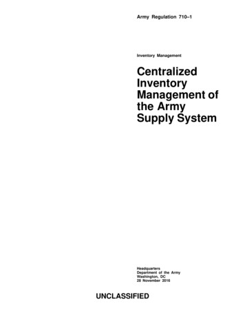
S. SinghFigure 1. Inventory order cycle of EOQ model.ordering cost per order is 5 and the carrying cost is 0.025 of the average inventory value. The price of a single unit is two hundred. The company presently hasa policy of placing ten orders every year: Advise the management of MonuTractors as to whether it should continue with its present policy or switch overto EOQ model.Here D 50000; Ordering Cost 5; Carrying Cost 2.5%; Cost Price 200.The model built here has considered both the cases i.e. carrying cost is constant or dependent on the holding cost.Excel Program of Economic Order Quantity Model (Figure 2 and Figure 3).AssumptionsIt’s an extension of EOQ model, in this, items are not received instantaneously. Supposition that Order quantity is received all at once is relaxed. The demandof the item is not high enough to warrant continuous production. Thereforeitems are produced in lots or batches.p—Daily production rate; d—Daily demand rate; D Annual Demand; Cs Set up Cost; Cc Carrying Cost.Annual Production rate (P) is more than the annual demand (D).Maximum inventory level at any time in the production cycle is given byQ— Q d p Q (1 d p )Q(1 d p ) .22Cs DOptimal Production Quantity Qopt . d CC 1 p Mean Inventory Level is given byLike previous model, total cost is sum of the set up cost and holding costTotal Cost Cs D Cc Q d 1 Q2 p Case II: XYZ (p) Ltd. is the sole bottler of Coca Cola at the Central India. Theannual demand of Pepsi at Nagpur is 2,000,000 bottles. The CC of the inventoryof bottled Coca cola is 10 per bottle per year. The set-up cost per bottling run is 1000. The rate of production is 10,000 bottles per day and the rate of demand is6000 bottles per day. Find the optimum size of a bottling run, i.e., the number ofbottles that should be manufactured in one production run.DOI: 10.4236/tel.2018.8111372097Theoretical Economics Letters

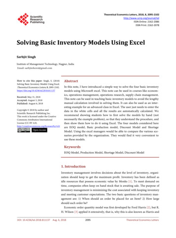
S. SinghFigure 2. Solution using excel for case I (Example of EOQ Model).Figure 3. Economic production quantity.Here Annual Demand is 2 million, the holding cost is ten dollars per bottleper year, the cost of setting up the production is 1000 and daily production p 10,000 bottles and daily demand 6000 bottles.The model built has considered both the cases of carrying cost i.e. it is constant or dependent on the price of the item.Excel Program for solving Production Quantity Model (Figure 4 and Figure 5).In most of the practical scenarios the unit cost of an item is dependent on thequantity procured. Mostly, discounts are offered for the purchase of large quantities. These discounts take the form of price breaks.Price per unit decreases as order quantity increases.In this case total cost includes the purchasing cost also.First step is to check the EOQ by using the EOQ formula and then check thetotal cost at the price breaks, whichever gives the lowest the optimal orderingquantity. Here p is the cost price and D is the annual demand.Total Cost Ordering Cost Carrying Cost Purchasing CostTotal Cost Co * D/Q Co * D/Q p * DDOI: 10.4236/tel.2018.8111372098Theoretical Economics Letters

S. SinghFigure 4. Solution of the case II using excel program.Figure 5. Quantity discount model.Case III A factory needs 200items, carrying cost 20%, ordering cost 100.Price break:0 - 2999; 10;3000 - 5000; 9.25;5000 & above; 8.75.Find the optimal lot size and the total inventory cost.Excel Program for solving quantity discount model (Figure 6 and Figure 7).In this model is demand is constant over the finite time horizon and supply isinstantaneous. Shortages are allowed and are fully backloggedQ total demand per production runHere in this model one more cost is involved i.e. shortage cost. The shortagecost is denoted by CshOptimal Ordering Quantity Qopt 2 DCoCcCc CshCsh Csh Maximum Inventory Level M Qopt Csh Cc DOI: 10.4236/tel.2018.8111372099Theoretical Economics Letters

S. SinghFigure 6. Solution of the case III using excel program.Figure 7. Deterministic Inventory problem with allowable shortages.Allowable Shortages are given by S Qopt M .Total Inventory Cost is the sum of ordering cost, holding cost and shortagecost.Total Inventory Cost 2DCo Cc M 2 Csh (Qopt M ) Qopt2Qopt2QoptCase IV:A dealer has to supply his customer 24,000 units of his product every year.The demand is fixed and known. The penalty of not meeting the demand istwenty cents per month. The inventory holding cost is ten cents per unit permonth and the ordering cost is 350 per order. Find the optimal order quantitywith allowable shortages. The allowable shortages and the total cost. Also compare with the EOQ model.Excel Program for Allowable Shortage Model (Figure 8 and Figure 9).DOI: 10.4236/tel.2018.8111372100Theoretical Economics Letters

S. SinghFigure 8. Solution of case IV considering allowable shortages.Figure 9. Concluding remarks.The excel programs given above would help the students to do the analyses ofthe various situations. For example comparison of the company present policywith applicable inventory model. Whether the company should opt for the discount offered by the supplier. It would be a wise decision to produce the item oroutsource. Also, companies should go for shortages or not. Thus, by making theabove programs, students can do analysis at a faster and easier way. The programs considered above have tried to cover all the aspects of the Inventory model like it provided the option whether carrying cost is constant or dependent onthe average inventory. Similarly, daily demand and production rate is given orannual demand and production rate. Accordingly the model can calculate thedaily demand and production rate. First student should be introduced to the basic models and then they should be provided these excel programs to do furtheranalysis.Conflicts of InterestThe authors declare no conflicts of interest regarding the publication of this paper.ReferencesDOI: 10.4236/tel.2018.811137[1]Monks, J.G. (1987) Operations Management. 3rd Edition, Theory and Problems.McGraw-Hill Book Co., New York.[2]Harris, F.W. (1915) Operations Cost (Factory Management Series). Shaw, Chicago.2101Theoretical Economics Letters

S. SinghDOI: 10.4236/tel.2018.811137[3]Wilson, R.H. (1934) A Scientific Routine for Stock Control. Harvard Business Review, 13, 116-128.[4]Davis, R.C. (1931) Purchasing and Storing, Alexander Hamilton Institute, NewYork.[5]Hadley, G. and Whitin, T.M. (1963) Analysis of Inventory Systems. Prentice-Hall,Englewood Cliffs, N.J.[6]Cargal, J.M. (2003) The EOQ Inventory Formula. Mathematical Sciences, 1.31, Ed.[7]Piasecki, D. (2009) Inventory Management ical Economics Letters

Solving Basic Inventory Models Using Excel Sarbjit Singh Institute of Management Technology, Nagpur, India Abstract In this note, I have introduced a simple way to solve the four basic inventory models using Microsoft excel. This note can be used in courses like econom-ics, operations management, operations research, supply chain management.