Transcription
CHAPTERFOUROPERATf ONAL-AMPLIFIER CIRCUITSThe operational anzplifier (op amp) is an extremely versatile and inespensivesemiconductor device. It is the workhorse of the communication. control. andinstrumentation industry.For low-fiqrtency applications, the op amp behaves like a four-terminalnonlinear resistor which can often be represented by an ideal up-amp model.This model greatly simplifies the analysis and design of op-amp circuits. In fact,one of the reasons why op amps are so popular is that. at low frequencies, theybehave almost like the ideal model! Consequently. except in the last section.our methods of analysis in this chapter will be based on the ideal model. Thischoice is justified in Sec. 4 by analyzing a typical op-amp circuit (operating atlow frequency) using a more complicated (finite-gain) op-amp model and thencomparing the results with those predicted by the ideal op-amp model.Depending on the dynamic range of the input signals, an op amp mayoperate in the linear or nonlinear region. Section 2 is devoted to those circuitswhere the op amp is operating only in the linear region. This restriction allowsus to simplify the (nonlinear) ideal op-amp model into a linear model. calledthe virtual short-circuit model. This model is used exclusively in Sec. 2 foranalyzing both simple circuits by inspection, as well as complicated circuits viaa systemaric method.The organization in Sec. 2 is followed in Sec. 3 for op amps operating inthe nonlinear region. Here, it is necessary to use the (nonlinear) ideal op-ampmodel.1 DEVICE DESCRIPTION, CHARACTERISTICS, AND MODELOperational amplifiers (op amps) are multiterminal devices sold in severalstandard packages, two of which are shown in Figs. 1.1 and 1.2. Because they
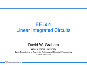
E(b)Figure 1.1 Eight-lead metal can. ( a ) Sideview. ( h ) Top view.Figure 1.2 A 14-lead DIP (dual in-line package). (a) Side view (b) Top view.are inexpensive (some cost less than 25 cents a piece), reliable, and extremelyversatile, op amps have become the workhorse of the electronics industry.Over 2000 types of integrated circuits ( I C ) op amps are currently available,each containing nearly two dozen transistors. Figure 1.3 gives the schematic ofthe popular pA741, a second-generation op amp introduced by FairchildSemiconductor in 1968. The seven terminals brought out through the packageleads are labeled inverting input, noninverting input, output, E , E-, andoffser nuN (two of them). The remaining terminals of the package in Figs. 1.lband 1.2b not connected to the IC are labeled NC (for no connection).Some op amps have more than seven terminals; others have less. For mostapplications, however, only the five terminals indicated in the standard op-ampsymbol in Fig. 1.4a are essential. The additional terminals are usually connected to some external nuliing or compensation circuit for improving the performance of the op amp. In order for the op amp to function properly its internaltransistors must be biased at appropriate operating points. Terminals E andE- are provided for this purpose. In general, they are connected to a splitpower supply as shown in Fig. 1.4b, where E and E- denote the voltagewith respect to the external ground. Typically, E 15 V and E- - 15 V.
InvertinginputTOffset nullFigure 1.3 Schematic of the pA74l op round(b)Figure 1.4 Standard op-amp symbol and a typical biasing scheme. (a) The - and -i- signs inside thetriangle denote the inverting and noninverting input terminals, respectively. ( b )A "biased" o p amp(enclosed within the triangle) can be considered as a 4-terminal device for circuit analysis and designpurposes.
After the power supply has been connected and after an external nuHingand/or compensation circuit has been connected to any additional terminals,only four terminals are available for external connections. Hence, from thecircuit designer-S point of view. an op amp is really a four-terminal device,regardless of the originai number of terminals in the op-amp package. Thisfour-terminal device Iies inside the dotted triangle in Fig. l.4b and willhenceforth be denoted by the symbol shown in Fig. 1.5a.l Here, i- and i,denote the current entering the op-amp "inverting" and "noninvetting" terminals. respectively. Similarly. v-. v,. and U, denote respectively the voltageand output terminalfrom the inverting terminal G,noninverting terminal 0,A@ to ground. The variable v , v - v - is called the differential I'npnr volrageand will plav an important roIe in op-amp circuit anaIysis.To derive an exact characterization of an op amp would require analyzingthe entire integrated circuit. such as the one shown in Fig. 1.3. Fortunately, formany low-frequency applications, the op-amp terminal currents and voltageshave been found usperimerzrall to obey the following nppro.uimnre relationships:where 1,- and 1,- are called the input bias currents and f(u,) denotes thev,-vs.-U, transfer characteristic. Apart from a scaling factor which depends onthe power supply voltage, f(v,,) follows approximately an odd-symmetricvv,.Ew (b)Figure 1.5 Experimental characterization of a typical op amp.' The op-amp symbol given in most electronics literature shows only three terminals with theground terminal omitted. This is because the ground terminal in Fig. 1.4b does not exist physicallyas a pin in most modem op-amp packages, but is rather created externally through the dual powersupply. We added this terminal because without it, KCL would give the erroneous relationshipi- i i, O.
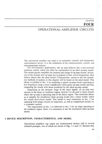
OPERATIONAL-AMPLIFIER CIRCUITS175function as shown in Fig. 1.5b (drawn for a t15-V supply voltage). Moreover,this function has been found to be rather insensitive to changes in the outputcurrent i, .The transfer characteristic in Fig. 1.5b displays three remarkable properties:1. v, and U, have different scales: one in volts, the other in millivolts.2. In a small interval - E ud E of the origin, f(v,,) * A V , is nearly linearwith a very steep slope A-called the open-loop volrage gain.3. f(v,) saturaies at v, r E,,,, where E,,, is typically 2 V less than the powersupply voltage (E,,, 13 V in Fig. 1.5b).In most op amps using bipolar input transistors, such as in Fig. 1.3,1,- andI,, represent the dc base currents used to bias the transistors (typically, lessthan 0.2 mA). For op amps using FET input transistors, the input bias currentsare much smaller. For example, the average input bias current I , (jIB,l ] 1,- 1) is equal to 0.1 mA for the pA741 but only 0.1 nA for the pA740 (whichuses a pair of FET input transistors).The open-loop voltage gain A is typically equal to at least 100.000 (200.000for the pA741). On the other hand, the voltage E at the end of the linearregion in Fig. 1.5b is typically less than 0.1 mV.An ideal op-amp model In view of the typical magnitudes of I, - . I, , A , andE , little accuracy is lost by assuming I,- I, E 0 and A X . Thissimplifying assumption leads to the ideal op-amp model shown in Fig. 1.6a andb. Note that the transfer characteristic f(v,) in this ideal model has beenapproximated by a three-segment piecewise-linear characteristic. For futurereference, the three distinct operating regions are labeled Linear, Saruration,and - Saturation, respectively, in Fig. 1.6.To emphasize that A r: in the linear region, we add X inside the triangle other models. Unlessto distinguish the ideal op-amp symbol in Fig. 1 . 6 fromotherwise stated, this ideal op-amp model will be used throughout this book.The ideal op-amp model can be described analytically as follows: Equationsdescribingthe idealOP- "PmodelBecause these equations are rather cumbersome and difficult to manipulateanalytically, it is much more practical to represent each region by a simpleequivalent circuit, as shown in Fig. 1.6c, d , and e, respectively.Note that these three equivalent circuits contain exactly the same information as Eq. (1.2). In particular, when the op amp is operating in the linear
invertinginputSoninvertinginput:l!ai- O- 0-C0i ot r ) EquivaIcnt circuitfor linear region--1I( d ) Equivalent circuitfor Saturation region(P)Equivalent circuitfor - Saturation regionFigwe 1.6 Ideal op-amp model.region. the ideal op-amp model reduces to that shown in Fig. 1 . 6 Note.thathere. v, is constrained to be zero at all times while (U,] is constrained to be lessthan the saturation voltage E,,,. Hence, this circuit is described by Eqs. (1.2a),(1.2b), and ( 1 . 2 d ) .The circuit in Fig. 1.6d is described by Eqs. ( 1 . 2 ) .(1.2b), and ( 1 . 2 )withv, O. Likewise, the circuit in Fig. 1.6e is described by Eqs. (1.2a), (1.2b).and ( 1 . 2 )with v, O .The ideal op-amp model is therefore described by three equivalent circuits,one for each operating region. If an op amp is known, a priori, to be operatingin only one of these three regions in a given circuit, then we sometimes abuseour fanguage by referring to the corresponding equivalent circuit in Fig. 1.6 asthe ideal op-amp model.For most low-frequency applications, the ideal op-amp model has beenfound to be quite reaiistic. For some specialized low-frequency applications(such as precision instrumentation) or high-frequency applications (such asfilters), various op-amp imperfections may become important. In that case, theideal model can be refined by introducing additional circuit elements.Most op-amp circuits are designed so that the op amps operate only in thelinear region. These circuits may contain both linear and nonlinear elements,and are studied in Sec. 2 using the equivalent circuit in Fig. 1 . 6 .Otherop-amp circuits are designed to take advantage of the abrupt nonlinearities andare studied in Sec. 3 using all three equivalent circuits in Fig. 1.6.
OPERATIONAL-AMPLIFIER CIRCUITS177Exercises1. The op-amp manufacturers' data sheets usually specify the typical valueof the average input bias current I , A ( / I B I 11,- I) and the &er currentAI,, /I,,[- /I,-I. Express IIB I and II,-I in terms of I , and I,,.2. Calculate I,- and I,- for the following op amps:fiA709Typical input biascurrent at 25 CLMlOlpA741LXI3OlALMlOlA70 nA30 nAZOO nA120nA80 nA50 nA40 nA20 nATypical offset currentat 25'C3.0 nA1.5 nA3. The data sheet for the @A741shows a typical open-loop voltage gain of200,000. Calculate the value of E for the following power supply voltages(assume E,,, magnitude of power supply voltage - 2 V): ( a ) 15 V and (b)220 v.2 OP-AMP CIRCUITS OPERATING IN THE LINEAR REGIONThe methods to be developed in this section are valid only if the op-ampoutput voltage satisfiesfor all times t (see Fig. 1.6b). We will henceforth refer to the expression (2.1)as the validating inequality for the linear region. If this inequality is violatedover any time interval [ t , , t , ] , the solution in this interval is incorrect and mustbe recalculated using the method in Sec. 3.2.1 Virtual Short Circuit ModelRecall from Chap. 3 that a three-port or four-terminaI resistor is characterizedby three relationships among the associated voltage and current variables. Inthe linear region, the ideal op-amp model in Fig. 1 . 6 and b can be describedanalytically by three equationx2Vialshort circuitmodelConsequently, we can think of the ideal op-amp model in Fig. 1 . 6 as athree-port or four-terminal resistor. For purposes of analysis, Eq. (2.2) is'These correspond to Eqs. (1.2a), (1.2b), and (1.2d).
B78LINEAR A N D NONLINEAR CIRCUITSequivalent to ( a ) connecting a short circuit across the op-amp input terminals,and ( b )stipulating that rhe current through it is Z P X O SIC nil times. T o emphasizethe special nature of this short circuit, we will henceforth refer to Eq. (2.2) asthe virt lraishort circrtit model. Using this equivalent circuit, many op-ampcircuits can be analyzed by inspection.2.2 Inspection MethodThis method usually requires no more than three calculations and is oftenimplemented by invoking KCL and Eq. (1.2) mentally with perhaps anoccasional scribble on the "back of the envelope." It is best illustrated viasome useful op-amp circuits as examples.A. Voltage 'follower (buffer) The simplest op-amp circuit operating in the linearregion is the voltage follower shown in Fig. 2.ln. To illustrate the inspectiorzmethod, we first apply KCL at node @ and obtainiin- i- 0(2.3)Applying next KVL around the closed node sequence @-@-@weobtain v,, - v,, U,, 0. Since v,, 0, we haveTo complete the analysis, we apply the validrrting inequahy (2.1) andobtain- E,,, U," E,,,(2.5)This gives the dynamic range of input voltages beyond which the op amp nolonger operates in the linear region.Note that Eqs. (2.3) and (2.4) define a unity-gain VCVS (Fig. 2.1 b). Thiscircuit has an infinite input resistance because ii, 0 and its output "duplicates" the input voltage, regardless of the external load. Consequently, it isFigure 2.1 The voltage follower circuit in ( a ) is equivalent to the unity-gain VCVS in ( b ) .
OPERATIONAL-AMPLIFIER CIRCUITS179usually called a voltage follower, a buffer. or an isol tionamplifier. It is widelyused between 2 two-ports as shown in Fig. 2.2 to prevent IV, from "loadingdown" N,. This isolation technique is one of the most useful tools in thedesigner's bag of tricks.Exercises1. ( a ) Let h.', and N , denote two identical linear voltage dividers made ofresistances R , and R,. Find the transfer characteristic v(, f(uin). ( b )Repeat (a) without ihe buffer.2. ( a ) Let N I and iY, denote the "half-wave rectifier circuit" (Fig. 6.3a)analyzed earlier in chap. 2. Find the v,, vs. vi, transfer characteristic. (b)Does your answer from ( a ) remain valid if N I is connected directly to A',?B. Inverting amplifier To illustrate the inspection method for op-amp circuitscontaining linear resistors. consider the circuit shown in Fig. 3.3. Since v, 0,we have U , v,,, and hence i , ui,/R , . Since i- 0. we have i, i l , andhence v, Rfi, Rf(vi,IR,). Applying KVL around the closed node sequencewe obtain@-@-a-@,Figure 2.2 The above buffer greatly simplifies analysis and allows h', and N , to be designedseparately.Figure 2.3 An inverting amplifier.
Substituting Eq. (2.6) into the validating inequality (2.1) and solving forv,,, we obtain the dynamic rangefor which Eq. (2.6) is valid.Hence. so long as the input signal satisfies Eq. (2.7), this circuit functionsas a voltage amplifier with a voltage gain equal to - R,/R, (assuming Rf R,).Note that the negative sign means that for a sinusoidal input, the output isshifted in phase by 180". Consequently, this circuit is called an invertingamplifier. In the special case where R, R,, it is called a phase inverter.(Why?)Note that whereas i- 0 and i O are imposed by the op-amp v-icharacteristics. the "virtual short circuit" v, 0 is achieved externally by"feeding back" the output voltage v, to the op-amp inverting terminal throughthe feedback resistor R,. The physical mechanism which automatically adjustsv, to a nearly zero voltage is discussed in Sec. 3.2B.Exercises1. Using a buffer and the circuit in Fig. 2.3 (assume R, 10 K), design aVCVS (c, pv,,) with a controlling coefficient p -1000.2. Repeat Exercise 1 with p 1000. Hint: Add a phase inverter.C. Noninverting amplifier As a further iIlustration of the inspection method,consider next the circuit shown in Fig. 2.4. Since v, 0, we have v, v;,, andhence i, v,,/R,. Since i- 0, we have i, i, vi,/R,, and hence v, ( R f l R,)vi,. Applying KVL around the closed node sequenceandsimplifying, we obtain@-@a-@0Figure 2.4 A noninverting amplifier.C
OPERATIONAL-AMPLIFIERCIRCUITS181Substituting Eq. (2.5) in the validating inequality (2.1) and solving for vi,,we obtain the dynamic rangefor which Eq. (2.5) is a l i d .Hence. so long as the input signal satisfies Eq. (2.9). this circuit functionsas a voltage amplifier Lvith a positive voltage gain ( R , R,.)IR,. It is usuallycalled a rzoninl-erring arnpl er. Note that a voltage follower is simply aunity-gain noninverting amplifier obtained by choosing R , X and R f 0.Exercises1. The circuit in Fig. 2.5 is called an algebraic srtntrner because v, k , v , k , v , . Find k and k , and identify the region in the U,-v, plane forwhich this-relationship is vilid.2. Using exactly trvo o p amps and n 3 resistors. design an n-inputsummer giving U,, v , v, - - v,,.3. ( a ) Explain why the resistor R, in Figs. 2.3 and 2.4 can be replaced byany one-port (except an open circuit) without affecting the value of i,. (b)Using a 3-V battery and either circuit in Figs. 2.3 and 2.1. design a dccurrent source having a terminal current of 30 mA. Hint: Use the propertyfrom ( a ) . ( c ) Repeat ( b ) for a terminal current of -30 mA.4. Using only one op amp and one resistor, design a VCCS described byi, kvi,, where k 0. Specify the maximum range of permissible "load"voltage across the current source.D. Resistance measurement without surgery T o show that the "virtual shortcircuit" is not just a powerful tool for simplifying analysis, Fig. 2.6 gives acircuit which exploits this remarkable property in a practical design. The linearresistive circuit enclosed within the circle represents the portion of a circuitwhere the value of each resistance is to be measured without cutting any wires.This problem usually arises when a circuit breaks down and a faulty resistor ist o be identified by comparing its resistance with the nominal value.Figure 2.5 An algebraic summer
182 LINEAR A N D NONLIWEAR CIRCUlTSFigure 2.6 An op-amp fault detector.To show how this circuit works, suppose resistor R, is to be measured. (a)Connect the op-amp inverting terminal @ to one terminal of Rj (node @ inFig. 2.6) and ground the second terminal of all other resistors connected toand @ in Fig. 2.6). (b) Connect the op-amp outputnode @ (nodes m, 0.terminal @ to the second terminal of Rj (node @ in Fig. 2.6). It follows fromthe virtual short-circuit property that except for Ri, the current through allresistors connected to node @ is zero. Moreover, since i, EIR and i- 0, wehave i, EIR and 0, (EIR)R,. Hence, by measuring the voltage v,, we cancalculateNote that without the virtual short circuit, R j would have to be cut before itsvalue can be measured.E. Nonlinear feedback To illustrate that the inspection method holds even ifthe op-amp circuit contains one or more nonlinear resistors, consider the circuitshown in Fig. 2.7. By inspection, we note that i, i, vinlRIand v, -v,.Figure 2.7 An op-amp circuitcontaining a nonlinear resistor.
OPERATIONAL-AMPLIFIER CIRCUITS183ConsequentlyTo determine the dynamic range of vi, for which Eq. (2.11) holds, we applythe validating inequality (2.1) and obtainEquations (2.11) and (3.12) give the nonlinear transfer characteristic withthe op amp operating in the linear region. Since this configuration is widelyused in nonlinear applications, we will consider an example.Example Let R , 1 klCl in Fig. 2.7. Let the nonlinear resistor represent theone-port shown in Fig. 2.8a. Using the graphic method from Chap. 2. weobtain the driving-point characteristic in Fig. 2.8b. where we have chosenv, as the vertical axis so that the curve represents v, f(i,). It follows fromE . (2.11) that the transfer characteristic is obtainid by flipping this curveabout the horizontal axis and then relabeling v, and i, with v, and v,,,respectively. The result is shown in Fig. 2 . 8 .Assuming a 15-V supply voltage for the op amp so that E,,, 13 V, wenote that Eq. (2.12) is satisfied for all values of v,, because Iv,l I-f(v,,l ,)I 10 V in Fig. 2 . 8 Hence,.we have demonstrated that the opamp can operate in the linear region for all values of input voltages, eventhough the circuit contains two nonlinear devices (zener diodes in thisexample).An examination of Fig. 2 . 8 shows that all input signal amplitudesexceeding 5 V will give a constant output of 210V. Consequently, thecircuit in this example is called a limiter or clipper, and is widely used forovervoltage protection and other applications in communication circuits.l 0 V zenerdiode2kSZi2 a 'b v--6Figure 2.8 (a) Circuit for realizing the nonlinear resistor 9?2 in Fig. 2.7. ( b ) Driving-pointcharacteristic of the circuit in a. (c) Transfer characteristic of the circuit in Fig. 2.7 with 92replaced by the circuit in a, and assuming R , l kQ.
184LINEAR AND NONLINEAR CIRCUITS2.3 Systematic MethodThe izzspectior method often fails whenever it is necessary to solve two ormore simultaneous equations. In such cases, it is desirable to develop asvstemntic ?zzerlrori for writing a system of linearly independent equationsinvolving as few roriables as possible. The following example illustrates thebasic steps involved.Example Consider the op-amp circuit shown in Fig. 2.9. where the op ampis modeled by a virtual short circuit (Fig. 1.6 ).Although this circuit couldbe solved by inspection. we will solve it by the systematic method, and letthe reader verify its answer by the inspection method.Step I. LabeE the nodes consecutively and f t e, denote as usual the voltagefrom nodeto datum. j 1 . 2 , . . . - 5 . Express all resistor voltagesand the differential op-amp voltage v, in terms of node-to-datumvoltages via KVL:aSrep 2. Express the branch current in each linear resistor in terms ofnode-to-datum voltages via Ohm's law:'0Figure 2.9 An opamp circuit for illustrating the systematic method.I
Step 3. Identify all other branch current variables which cannot be expressed in terms of node-to-datum voltages, namely, the currents is, and is?of the voltage sources and the current i, of the op-amp outputterminal. Note that the op-amp input currents i- and I are notvariables (assuming an ideal op-amp model) because they are equal tozero. Our objective is to write a system of Iinearly independentequations in terms of the node-to-datum voltages {e,. e,. . . . .e,) andthe identified current variables {is,, i,, i,).Step 4. Write KCL at each node except the datum node in terms of. .{ e l , e2*e3, e4, e 5 . l s l , zs2, ia}:.Node Q:Node @:Node @:e1 - e3 i,, 0RIe* - e4 .--015, R3e3 - e5 e1 - e, - 0p-R2RINode @:e4R4Node @:I,e2 - e4 oR3e3 - e5 o-R2Step 5. Equation (2.15) consists of five equations with eight variables.Hence, we need to write three more independent equations. Since wehave already made use of KVL (Step l), KCL (Step 4), and theresistor characteristics (Step 2), these three equations must come fromthe characteristics of the voltage sources and the op amp:Voltage sources:Note that v, e, - e,.
186LINEAR AND NONLIWE.L\R CIRCUITSStep 6. Together. Eqs. (3.15) and (2.16) constitute a system of eightlinearly independent equations in terms of eight variables. Solvingthese equations for the desired op-amp output voltage e, by etimination and substitution of variables. or by any other method, we obtainNote that only Eqs. ( 2 . 1 5 and d ) and (3.16) are used to solve for U,,.The remaining equations (2.15a, b. and e ) are needed. however, tosolve for the remaining variables is,. l , , , and i,. respectively.Step 7. Determine the dynamic range of the input voltages where Eq.(2.17) holds. i.e. where the op amp is operating in the linear region:Hence. Eq. (3.17) holds at all times when the expression (2.18) is satisfied.Exercise Derive Eqs. (2.17) and (2.18) by the inspection method.Special case (differentia1 amplifier) Suppose R , / R , R,/R, in Fig. 2.9,Then Eqs. (2.17) and (2.18) reduce to the following:Equation (2.19) defines a differential dc amplifier, a circuit widely used ininstrumentation applications.The preceding systematic method is applicable to any op-amp circuitcontaining linear resistors, independent voltage and current sources, and opamps modeled by virtual short circuits. This method will be generalized inChap. 8 [called the modified node analysis ( M N A ) method] for arbitraryresistive circuits.Exercises1. Generalize the steps in the preceding systematic method for a connectedn-node circuit containing linear resistors, k voltage sources, f currentsources, and m op amps.2. ( a ) Show that in the linear region, the ideal op-amp model is equivalentto a linear two-port resistor described by a transmission matrix T whichspecifies the port variables v, and i- (associated with port 1) in terms ofthe port variables v, and i, (associated with port 2). (b) Use the"linearity" property from ( a ) to show any circuit made of linear resistors,independent sources, and ideal op amps operating in the linear region canbe analyzed by solving only linear equations.
OPERATIOAAL-AMPLIFIER CIRCUITS1873 OP-AMP CIRCUITS OPERATING IN THENONLINEAR REGIONThere are many applications where the op amp operates in all three regions ofthe ideal op-amp model in Fig. 1.6. This occurs whenever the amplitudes ofone or more input signals are such that the validating inequality in each regionis violated over some time intervals. In this case it is necessary to revert to thenonliriear model in Fig. 1.6 and we say the op amp is operating in the nonlinearregion. Fortunately. since the characteristic in Fig. 1.6b is pieceivise linear. thecircuit in each region can be easily analyzed as a linear circuit.3.1 Saturation and - Saturation Equivalent CircuitsIn the Saturation region, the ideal op-amp model in Fig. 1.6 can bedescribed analytically by three equations: SaturationcharacteristicsThese equations are applicable provided the following validating inequalit)?holds:Note that the crucial difference between the " Saturationcharacteristics" andAthe previous "linear characteristics" is that here, v, v, - v- # 0 and v, isnow "clamped" at a fixed positive voltage equal to E,,,. In this region, we canreplace the op amp by the equivalent circuit shown in Fig. 1.66, which isredrawn in Fig. 3.1 for convenience.Saturation region, the ideal op-amp model in Fig. 1.6 can beIn thedescribed analytically as follows:-- SaturationcharacteristicsFigure 3.1 The Saturation model.
188 LINEAR AND NONLINEAR CIRCUITSFigure 3.1 The - Saturation model.These equations are applicable provided the following validating inequaliryholds :(3.4)2,Again. in sharp contrast to the "linear characteristics." here U, v - v - f 0and U, is -'clamped" at a fixed negative voltage equal to -E,,,. In this region,we can replace the op amp by the equivalent circuit shown in Fig. 1.6e, whichis redrawn in Fig. 3.2 for convenience.Analogous to Eq. (2.11, we will henceforth call Eqs. (3.2) and (3.4) thevalidating ineqrrnlie for the Saruration and - Saturation regions, respectively.Corresponding to the three regions in the ideal op-amp model of Fig. 1.6,we have three simplified equivalent circuits defined by Eqs. (2.1) and (2.2),(3.1) and (3.21, and (3.3) and (3.41, respectively. The correct equivalent circuitto rise in a given situation depends on, and only on, which of the three validatinginequalities (2.1). (3.2), or (3.4) holds.3.2 Inspection MethodMost op-amp circuits which operate in the nonlinear region have a single inputand a single output of interest. For this class of circuits, the basic problem is toderive the driving-point characteristic or the transfer characteristic. Once thesecharacteristics are found, the output waveform due to any input waveform canbe easily obtained either graphically or by direct substitution. The method forderiving these characteristics is best illustrated via examples.A. Comparator (threshold detector) The simplest op-amp circuit operating inthe nonlinear region is the comparator circuit shown in Fig. 3.30. Replacingthe ideal op-amp model by the virtual short circuit, Saturation, and Saturation equivalent circuits, respectively, we obtain the corresponding linearcircuit shown in Fig. 3.4a, b, and c, respectively.Consider first the circuit in Fig. 3.4a. Since v, vin- E , 0, the op ampcan operate in the linear region if and only if vin ET.In such a case, we findii, O (Fig. 3.3b) and -E,,, v, C E,,, (Fig. 3 . 3 ) .Consider next the circuit in Fig. 3.4b. Since v, vin- E, 0, the op ampoperates in the Saturation region if and only if vin E,. In such a case, wefind iin 0 (Fig. 3.3b) and v, E,,, (Fig. 3 . 3 ) .
OPERATIONAL-AMPLIFIER CIRCUITS189i Int-E,,--SaturationLinear regionI / %antion SaturationLinearregionin- SaturationFigure 3.3 (a) Comparator. (b) Driving-point characteristic. (c) Transfer characteristic.-U,,iinv, iT :E,1Figure 3.4 Linear circuit for each region. oIeU0-E*,
1m LINEARA N D NONLINEAR CIRCUTTSIt remains to consider the circuit in Fig. 3 . 4 .Since v, v,, - E, 0, theo p amp operates in the - Saruration region if and only if U,, E,. In whichcase, we find i,,, D (Fig. 3.3b ) and U, - E,,, (Fig. 3 . 4 ) .An examination of the transfer characteristic in Fig. 3 . 3 shows that thecircuit "compares" the input signaI with a prescribed threshold voltage E, andresponds by jumping abruptly from one level to another. Consequently, it iscalIed a cornpnrafov or a threshold detector. In the special case where E, 0,the circuit becomes a zero-crossing defector. Comparators are so widely used indigital circuits that they are mass produced (with "bells and whistles" added forimproved performance) and soZd under the name "comparator."B. Negative vs. positive feedback circuit Consider the circuit shown in Fig.3.5a. Note that this is just the voltage follower in Fig. 2.1 studied earlier.There; we found that U,, v , , provided Iuin1 E,,,. By inspection, we foundU,, ES3,whenever uin) Eand v , -Es,, whenever v,, -E ,,,. The complete transfer characteristic is therefore as shown in Fig. 3.5b.This circuit is said to have a "negative" feedback because the outputvoltage is fed back to the inverting input terminaI.What happens if we interchange the inverting and noninverting terminalsas shown in Fig. 3.6a? By inspection, we found U, U,, provided / v , , [ E,,,.Hence, in the linear region, the transfer
linear region. These circuits may contain both linear and nonlinear elements, and are studied in Sec. 2 using the equivalent circuit in Fig. 1.6 . Other op-amp circuits are designed to take ad