Transcription
Hierarchical MatricesSteffen BörmLars GrasedyckApril 21, 2005Wolfgang Hackbusch
2
Contents1 Introductory Example (BEM)91.1Model Problem . . . . . . . . . . . . . . . . . . . . . . . . . . . . . . . . . . . . . . . . . . . .91.2Taylor Expansion of the Kernel . . . . . . . . . . . . . . . . . . . . . . . . . . . . . . . . . . .101.3Low Rank Approximation of Matrix Blocks . . . . . . . . . . . . . . . . . . . . . . . . . . . .121.4Cluster Tree TI . . . . . . . . . . . . . . . . . . . . . . . . . . . . . . . . . . . . . . . . . . . .131.5Block Cluster Tree TI I . . . . . . . . . . . . . . . . . . . . . . . . . . . . . . . . . . . . . . .141.6Assembly, Storage and Matrix-Vector Multiplication . . . . . . . . . . . . . . . . . . . . . . .161.6.1Inadmissible Leaves . . . . . . . . . . . . . . . . . . . . . . . . . . . . . . . . . . . . .161.6.2Admissible Leaves . . . . . . . . . . . . . . . . . . . . . . . . . . . . . . . . . . . . . .171.6.3Hierarchical Matrix Representation . . . . . . . . . . . . . . . . . . . . . . . . . . . . .18Exercises . . . . . . . . . . . . . . . . . . . . . . . . . . . . . . . . . . . . . . . . . . . . . . .191.7.1Theory . . . . . . . . . . . . . . . . . . . . . . . . . . . . . . . . . . . . . . . . . . . .191.7.2Practice . . . . . . . . . . . . . . . . . . . . . . . . . . . . . . . . . . . . . . . . . . . .201.72 Multi-dimensional Construction2.123Multi-dimensional cluster tree . . . . . . . . . . . . . . . . . . . . . . . . . . . . . . . . . . . .232.1.1Definition . . . . . . . . . . . . . . . . . . . . . . . . . . . . . . . . . . . . . . . . . . .232.1.2Geometric bisection . . . . . . . . . . . . . . . . . . . . . . . . . . . . . . . . . . . . .252.1.3Regular subdivision . . . . . . . . . . . . . . . . . . . . . . . . . . . . . . . . . . . . .262.1.4Implementation . . . . . . . . . . . . . . . . . . . . . . . . . . . . . . . . . . . . . . . .26Multi-dimensional block cluster tree . . . . . . . . . . . . . . . . . . . . . . . . . . . . . . . .322.2.1Definition . . . . . . . . . . . . . . . . . . . . . . . . . . . . . . . . . . . . . . . . . . .322.2.2Admissibility . . . . . . . . . . . . . . . . . . . . . . . . . . . . . . . . . . . . . . . . .322.2.3Bounding boxes . . . . . . . . . . . . . . . . . . . . . . . . . . . . . . . . . . . . . . . .332.2.4Implementation . . . . . . . . . . . . . . . . . . . . . . . . . . . . . . . . . . . . . . . .342.3Construction of an admissible supermatrix structure . . . . . . . . . . . . . . . . . . . . . .372.4Exercises . . . . . . . . . . . . . . . . . . . . . . . . . . . . . . . . . . . . . . . . . . . . . . .382.4.1Theory . . . . . . . . . . . . . . . . . . . . . . . . . . . . . . . . . . . . . . . . . . . .382.4.2Practice . . . . . . . . . . . . . . . . . . . . . . . . . . . . . . . . . . . . . . . . . . . .382.23
4CONTENTS3 Integral Equations413.1Galerkin discretization . . . . . . . . . . . . . . . . . . . . . . . . . . . . . . . . . . . . . . . .413.2Interpolation . . . . . . . . . . . . . . . . . . . . . . . . . . . . . . . . . . . . . . . . . . . . .423.2.1Degenerate approximation . . . . . . . . . . . . . . . . . . . . . . . . . . . . . . . . . .423.2.2Tensor-product interpolation on bounding boxes . . . . . . . . . . . . . . . . . . . . .433.2.3Construction of the low-rank approximation . . . . . . . . . . . . . . . . . . . . . . . .453.2.4Interpolation error bound . . . . . . . . . . . . . . . . . . . . . . . . . . . . . . . . . .45Example: Boundary Element Method in 2D . . . . . . . . . . . . . . . . . . . . . . . . . . . .473.3.1Curve integrals . . . . . . . . . . . . . . . . . . . . . . . . . . . . . . . . . . . . . . . .473.3.2Single layer potential . . . . . . . . . . . . . . . . . . . . . . . . . . . . . . . . . . . . .483.3.3Implementation . . . . . . . . . . . . . . . . . . . . . . . . . . . . . . . . . . . . . . . .49Exercises . . . . . . . . . . . . . . . . . . . . . . . . . . . . . . . . . . . . . . . . . . . . . . .503.4.1503.33.4Practice . . . . . . . . . . . . . . . . . . . . . . . . . . . . . . . . . . . . . . . . . . . .4 Elliptic Partial Differential Equations4.153One-Dimensional Model Problem . . . . . . . . . . . . . . . . . . . . . . . . . . . . . . . . . .534.1.1Discretization . . . . . . . . . . . . . . . . . . . . . . . . . . . . . . . . . . . . . . . . .534.1.2The Stiffness Matrix in H-Matrix Format . . . . . . . . . . . . . . . . . . . . . . . . .544.1.3The Inverse to the Stiffness Matrix in H-matrix Format . . . . . . . . . . . . . . . . .554.2Multi-dimensional Model Problem . . . . . . . . . . . . . . . . . . . . . . . . . . . . . . . . .564.3Approximation of the inverse of the stiffness matrix . . . . . . . . . . . . . . . . . . . . . . . .584.3.1Notation of Finite Elements and Introduction into the Problem . . . . . . . . . . . . .584.3.2Mass Matrices . . . . . . . . . . . . . . . . . . . . . . . . . . . . . . . . . . . . . . . .594.3.3Connection between A 1 and B. . . . . . . . . . . . . . . . . . . . . . . . . . . . . .624.3.4Green Functions . . . . . . . . . . . . . . . . . . . . . . . . . . . . . . . . . . . . . . .634.3.5FEM Matrices . . . . . . . . . . . . . . . . . . . . . . . . . . . . . . . . . . . . . . . .69Implementation . . . . . . . . . . . . . . . . . . . . . . . . . . . . . . . . . . . . . . . . . . . .714.4.1Sparse Matrices . . . . . . . . . . . . . . . . . . . . . . . . . . . . . . . . . . . . . . . .714.4.2Assembly of Stiffness and Mass Matrices . . . . . . . . . . . . . . . . . . . . . . . . . .74Exercises . . . . . . . . . . . . . . . . . . . . . . . . . . . . . . . . . . . . . . . . . . . . . . .764.5.1Theory . . . . . . . . . . . . . . . . . . . . . . . . . . . . . . . . . . . . . . . . . . . .764.5.2Practice . . . . . . . . . . . . . . . . . . . . . . . . . . . . . . . . . . . . . . . . . . . .764.44.55 Arithmetics of Hierarchical Matrices5.15.277Arithmetics in the rkmatrix Representation . . . . . . . . . . . . . . . . . . . . . . . . . . . .775.1.1Reduced Singular Value Decomposition (rSVD) . . . . . . . . . . . . . . . . . . . . . .785.1.2Formatted rkmatrix Arithmetics . . . . . . . . . . . . . . . . . . . . . . . . . . . . . .80Arithmetics in the H-Matrix Format . . . . . . . . . . . . . . . . . . . . . . . . . . . . . . . .82
CONTENTS5.355.2.1Addition and Multiplication . . . . . . . . . . . . . . . . . . . . . . . . . . . . . . . . .825.2.2Inversion . . . . . . . . . . . . . . . . . . . . . . . . . . . . . . . . . . . . . . . . . . .875.2.3Cholesky and LU Decomposition . . . . . . . . . . . . . . . . . . . . . . . . . . . . . .88Exercises . . . . . . . . . . . . . . . . . . . . . . . . . . . . . . . . . . . . . . . . . . . . . . .905.3.1Theory . . . . . . . . . . . . . . . . . . . . . . . . . . . . . . . . . . . . . . . . . . . .905.3.2Practice . . . . . . . . . . . . . . . . . . . . . . . . . . . . . . . . . . . . . . . . . . . .906 Complexity Estimates6.16.26.36.493Arithmetics in the rkmatrix Representation . . . . . . . . . . . . . . . . . . . . . . . . . . . .936.1.1Reduced Singular Value Decomposition (rSVD) . . . . . . . . . . . . . . . . . . . . . .936.1.2Formatted rkmatrix Arithmetics . . . . . . . . . . . . . . . . . . . . . . . . . . . . . .94Arithmetics in the H-Matrix Format . . . . . . . . . . . . . . . . . . . . . . . . . . . . . . . .946.2.1Truncation . . . . . . . . . . . . . . . . . . . . . . . . . . . . . . . . . . . . . . . . . .966.2.2Addition . . . . . . . . . . . . . . . . . . . . . . . . . . . . . . . . . . . . . . . . . . . .976.2.3Multiplication . . . . . . . . . . . . . . . . . . . . . . . . . . . . . . . . . . . . . . . . .976.2.4Inversion . . . . . . . . . . . . . . . . . . . . . . . . . . . . . . . . . . . . . . . . . . . 101Sparsity and Idempotency of the Block Cluster Tree TI I . . . . . . . . . . . . . . . . . . . . 1026.3.1Construction of the Cluster Tree TI . . . . . . . . . . . . . . . . . . . . . . . . . . . . 1026.3.2Construction of the Block Cluster Tree TI I . . . . . . . . . . . . . . . . . . . . . . . 103Exercises . . . . . . . . . . . . . . . . . . . . . . . . . . . . . . . . . . . . . . . . . . . . . . . 1056.4.1Theory . . . . . . . . . . . . . . . . . . . . . . . . . . . . . . . . . . . . . . . . . . . . 1057 H2 -matrices1077.1Motivation . . . . . . . . . . . . . . . . . . . . . . . . . . . . . . . . . . . . . . . . . . . . . . 1077.2H2 -matrices . . . . . . . . . . . . . . . . . . . . . . . . . . . . . . . . . . . . . . . . . . . . . . 1087.2.1Uniform H-matrices . . . . . . . . . . . . . . . . . . . . . . . . . . . . . . . . . . . . . 1087.2.2Nested cluster bases . . . . . . . . . . . . . . . . . . . . . . . . . . . . . . . . . . . . . 1107.2.3Implementation . . . . . . . . . . . . . . . . . . . . . . . . . . . . . . . . . . . . . . . . 1127.3Orthogonal cluster bases . . . . . . . . . . . . . . . . . . . . . . . . . . . . . . . . . . . . . . . 1147.4Adaptive cluster bases . . . . . . . . . . . . . . . . . . . . . . . . . . . . . . . . . . . . . . . . 1157.4.1Matrix error bounds . . . . . . . . . . . . . . . . . . . . . . . . . . . . . . . . . . . . . 1157.4.2Construction of a cluster basis for one cluster . . . . . . . . . . . . . . . . . . . . . . . 1167.4.3Construction of a nested basis . . . . . . . . . . . . . . . . . . . . . . . . . . . . . . . . 1177.4.4Efficient conversion of H-matrices . . . . . . . . . . . . . . . . . . . . . . . . . . . . . 1197.5Implementation . . . . . . . . . . . . . . . . . . . . . . . . . . . . . . . . . . . . . . . . . . . . 1197.6Exercises . . . . . . . . . . . . . . . . . . . . . . . . . . . . . . . . . . . . . . . . . . . . . . . 1207.6.1Theory . . . . . . . . . . . . . . . . . . . . . . . . . . . . . . . . . . . . . . . . . . . . 1207.6.2Practice . . . . . . . . . . . . . . . . . . . . . . . . . . . . . . . . . . . . . . . . . . . . 120
6CONTENTS8 Matrix Equations1238.1Motivation . . . . . . . . . . . . . . . . . . . . . . . . . . . . . . . . . . . . . . . . . . . . . . 1238.2Existence of Low Rank Solutions . . . . . . . . . . . . . . . . . . . . . . . . . . . . . . . . . . 1238.3Existence of H-matrix Solutions . . . . . . . . . . . . . . . . . . . . . . . . . . . . . . . . . . . 1248.4Computing the solutions . . . . . . . . . . . . . . . . . . . . . . . . . . . . . . . . . . . . . . . 1258.5High-dimensional Problems . . . . . . . . . . . . . . . . . . . . . . . . . . . . . . . . . . . . . 1279 Outlook9.1129Adaptive Arithmetics and Adaptive Refinement . . . . . . . . . . . . . . . . . . . . . . . . . . 1299.1.1Rank-adaptive Truncation . . . . . . . . . . . . . . . . . . . . . . . . . . . . . . . . . . 1299.1.2Adaptive Grid-Refinement . . . . . . . . . . . . . . . . . . . . . . . . . . . . . . . . . . 1299.2Other Hierarchical Matrix Formats . . . . . . . . . . . . . . . . . . . . . . . . . . . . . . . . . 1309.3Applications of Hierarchical Matrices . . . . . . . . . . . . . . . . . . . . . . . . . . . . . . . . 130Index9.3.1Partial Differential Equations . . . . . . . . . . . . . . . . . . . . . . . . . . . . . . . . 1309.3.2Matrix Functions . . . . . . . . . . . . . . . . . . . . . . . . . . . . . . . . . . . . . . . 130133
PrefaceA major aim of the H-matrix technique is to enable matrix operations of almost linear complexity. Therefore,the notation and importance of linear complexity is discussed in the following.Linear ComplexityLet φ : Xn Ym be any function to be evaluated, where n is the number of input data and m is the numberof output data. The cost of a computation is at least O(N ) with N : max{n, m}, provided that φ is anontrivial mapping (i.e., it is not independent of some of the input data and the output cannot equivalentlybe described by less than m data). If the cost (or storage) depends linearly on the data size N, we speakabout linear complexity. The observation from above shows that linear complexity is the optimal one withrespect to the order.Given a class of problems it is essential how the size N of the data behaves. The term “large scale computation” expresses that the desired problem size is as large as possible, which of course depends on the actualavailable computer capacity. Therefore, the size N from above is time-dependent and increases according tothe development of the computer technology.The computer capacity is characterised by two different features: the available storage and the speed ofcomputing. Up to the present time, these quantities increase proportionally, and the same is expected forthe future. Under this assumption one can conclude that large scale computations require linearcomplexity algorithms.For a proof consider a polynomial complexity: Let the arithmetical costs be bounded by CN σ for someσ 1. By the definition of a large scale computation, N Nt should be the maximal size suited forcomputers at time t. There is a time difference t so that at time t t the characteristic quantities aredoubled: Nt t 2Nt and speed t t 2speed t . At time t t, problems with Nt t data are to beσ C2σ Ntσ operations. Although the number of operations has increased by 2σ ,computed involving CNt tthe improvement concerning the speed leads to an increase of the computer by the factor 2 σ /2 2σ 1 . Ifσ 1 we have the inconvenient situation that the better the computers are, the longer are the running times.Therefore, the only stable situation arises when σ 1, which is the case of linear complexity algorithms.Often, a complexity O(N logq N ) for some q 0 appears. We name this “almost linear complexity”. Sincethe logarithm increases so slowly, O(N logq N ) and O(N ) are quite similar from a practical point of view.If the constant C1 in O(N ) is much larger than the constant C2 in O(N logq N ), it needs a very big Nt suchthat C2 Nt logq Nt C1 N, i.e., in the next future O(N logq N ) and O(N ) are not distinguishable.Linear Complexity in Linear AlgebraLinear algebra problems are basic problems which are part of almost all large scale computations, in particular, when they involve partial differential equations. Therefore, it is interesting to check what linear algebratasks can be performed with linear complexity.The vector operations (vector sum x y, scalar multiplication λx, scalar product hx, yi) are obvious candidates7
8CONTENTSfor linear complexity.However, whenever matrices are involved, the situation becomes worse. The operations Ax, A B, A B,A 1 , etc. require O(N 2 ) or O(N 3 ) operations. The O(N 2 )-case can be interpreted as linear complexity,since an N N -matrix contains N 2 data. However, it is unsatisfactory that one does not know whether a(general) linear system Ax b (A regular) can be solved by an O(N 2 )-algorithm.Usually, one is working with special subsets of matrices. An ideal family of matrices are the diagonal ones.Obviously, their storage is O(N ) and the standard operations Dx, D D 0 , D D0 , D 1 require O(N )operations. Diagonal matrices allow even to evaluate general functions: f (D) diag{f (d i ) : 1 i N }.The class of diagonal matrices might look rather trivial, but is the basis of many FFT applications. If,e.g., C is circulant (i.e., Cij Ci0 ,j 0 for all i j i0 j 0 mod N ), the Fourier transform by F leads toa diagonalisation: F 1 CF D. This allows to inherit all operations mentioned for the diagonal case tothe set of circulant matrices. Since the computation of Fx and F 1 x by the fast Fourier transform needsO(N log N ), these operations are of almost linear complexity. It is interesting to notice that F ω i j i,j 1,.,N with ω exp (2πi/N ) is neither stored nor used (i.e., noentries of F are called), when Fx is performed by FFT.Diagonalisation by other matrices than F is hard to realise. As soon as the transformation T to diagonal formis a full matrix and T x must be performed in the standard way, the complexity is too high. Furthermore,the possibility of cheap matrix operations is restricted to the subclass of matrices which are simultaneouslydiagonalised by the transformation.The class of matrices which is most often used, are the sparse matrices, i.e., #{(i, j) : A ij 6 0} O(N ).Then, obviously, the storage and the matrix-vector multiplication Ax and the matrix addition (in the samepattern) are of linear complexity. However, already A B is less sparse, the LU-decomposition A LUfills the factors L and U, and the inverse A 1 is usually dense. Whether Ax b can be solved in O(N )operations or not, is not known. The fact that Ax requires only linear complexity is the basis of most of theiterative schemes for solving Ax b.A subset of the sparse matrices are band matrices, at least when the band width ω is O(1). Here, LUdecomposition costs O(ω 2 N ) operations, while the band structure of A is inherited by the LU-factors. Thedisadvantages are similar to those of sparse matrices: A B has the enlarged band width ω A ωB and A 1is dense.The conclusion is as follows: As long as the matrix-vector multiplication x 7 Ax is the only desired operation, the sparse matrixformat is ideal. This explains the success of the finite element method together with the iterativesolution methods. Except the diagonal matrices (or diagonal after a certain cheap transformation), there is no class ofmatrices which allow the standard matrix operationsAx,in O(N ) operations.A B,A B,A 1
Chapter 1Introductory Example (BEM)In this very first section we introduce the hierarchical matrix structure by a simple one-dimensional modelproblem. This introduction is along the lines of [23], but here we fix a concrete example that allows us tocompute everything explicitly.1.1Model ProblemExample 1.1 (One-Dimensional Integral Equation) We consider the integral equationZ10log x y U(y)dy F(x),x [0, 1],(1.1)for a suitable right-hand side F : [0, 1] R and seek the solution U : [0, 1] R. The kernel g(x, y) log x y in [0, 1]2 has a singularity on the diagonal (x y) and is plotted in Figure 1.1.Figure 1.1: The function log x y in [0, 1] [0, 1] and a cut along the line x y 1.A standard discretisation scheme is Galerkin’s method where we solve equation (1.1) projected onto the(n-dimensional) space Vn : span{ϕ0 , . . . , ϕn 1 },Z10Z10ϕi (x) log x y U(y)dydx 9Z1ϕi (x)F(x)dx00 i n,
10CHAPTER 1. INTRODUCTORY EXAMPLE (BEM)and seek the discrete solution Un in the same space Vn , i.e., Un u is the solution of the linear systemGu f,Gij : Z10ZPn 1j 0uj ϕj such that the coefficient vector10ϕi (x) log x y ϕj (y)dydx,fi : Z1ϕi (x)F(x)dx.0In this introductory example we choose piecewise constant basis functions 1 if ni x i 1nϕi (x) 0 otherwise(1.2)on a uniform grid of [0, 1]:φ12001The matrix G is dense in the sense that all entries are nonzero. Our aim is to approximate G by a matrixG̃ which can be stored in a data-sparse (not necessarily sparse) format. The idea is to replace the kernelg(x, y) log x y by a degenerate kernelg̃(x, y) k 1Xgν (x)hν (y)ν 0such that the integration with respect to the x-variable is separated from the one with respect to the yvariable. However, the kernel function g(x, y) log x y cannot be approximated by a degenerate kernelin the whole domain [0, 1] [0, 1] (unless k is rather large). Instead, we construct local approximations forsubdomains of [0, 1] [0, 1] where g is smooth (see Figure 1.2).Figure 1.2: The function log x y in subdomains of [0, 1] [0, 1].1.2Taylor Expansion of the KernelLet τ : [a, b], σ : [c, d], τ σ [0, 1] [0, 1] be a subdomain with the property b c such that theintervals are disjoint: τ σ . Then the kernel function is nonsingular in τ σ. Basic calculus reveals
1.2. TAYLOR EXPANSION OF THE KERNEL11Lemma 1.2 (Derivatives of log x y ) The derivatives of g(x, y) log x y for x 6 y and ν N are xν g(x, y) ( 1)ν 1 (ν 1)!(x y) ν yν g(x, y) (ν 1)!(x y) ν .The Taylor series of x 7 g(x, y) in x0 : (a b)/2 converges in the whole interval τ , and the remainder ofthe truncated Taylor series can be estimated as follows.Lemma 1.3 (Taylor series of log x y ) For each k N the function (truncated Taylor series)k 1X1 ν x g(x0 , y)(x x0 )νν!ν 0g̃(x, y) : approximates the kernel g(x, y) log x y with an error g(x, y) g̃(x, y) x0 a c b 1 c b x0 a (1.3) k.Proof: Let x [a, b], a b, and y [c, d]. In the radius of convergence (which we will determine later) theTaylor series of the kernel g(x, y) in x0 fulfilsg(x, y) The remainder g(x, y) g̃(x, y) P X1 ν x g(x0 , y)(x x0 )ν .ν!ν 01 νν k ν! x g(x0 , y)(x X1 ν g(x0 , y)(x x0 )νν! x ν kν kSince 1 c b x0 a x0 )ν can be estimated by ν Xx x0ν 1 (ν 1)!( 1)ν!x0 y Xx x0 ν x0 yν k ν X x0 a x0 a c b ν k k x0 a c b 1 .1 c b x0 a 1, the radius of convergence covers the whole interval [a, b].If c b then the estimate for the remainder tends to infinity and the approximation can be arbitrarilybad. However, if we replace the condition b c, i.e., the disjointness of the intervals, by the strongeradmissibility conditiondist0τσ1diam(τ ) dist(τ, σ)(1.4)diamthen the approximation error can be estimated by g(x, y) g̃(x, y) 323(1 ) k 3 k .212(1.5)This means we get a uniform bound for the approximation error independently of the intervals as long asthe admissibility condition is fulfilled. The error decays exponentially with respect to the order k.
121.3CHAPTER 1. INTRODUCTORY EXAMPLE (BEM)Low Rank Approximation of Matrix BlocksThe index set I : {0, . . . , n 1} contains the indices of the basis functions ϕi used in the Galerkindiscretisation. We fix two subsets t and s of the index set I and define the corresponding domains as theunion of the supports of the basis functions:τ : [supp ϕi ,σ : [supp ϕi .i si tIf τ σ is admissible with respect to (1.4), then we can approximate the kernel g in this subdomain by thetruncated Taylor series g̃ from (1.3) and replace the matrix entriesZGij Pk 1by use of the degenerate kernel g̃ ν 0G̃ij : 10Z1ϕi (x)g(x, y)ϕj (y)dydx0gν (x)hν (y) for the indices (i, j) t s:Z10Z1ϕi (x)g̃(x, y)ϕj (y)dydx.0The benefit is twofold. First, the double integral is separated in two single integrals:G̃ijZ 10Z1ϕi (x)0k 1X Z 1 ν 0k 1Xgν (x)hν (y)ϕj (y)dydxν 0ϕi (x)gν (x)dx0 Z 1ϕj (y)hν (y)dy .0Second, the submatrix G t s can be represented in factorised formG t s AB T ,A Rt {0,.,k 1} , B Rs {0,.,k 1} ,ATBwhere the entries of the factors A and B areAiν : Z1ϕi (x)gν (x)dx,0Bjν : Z1ϕj (y)hν (y)dy.0The rank of the matrix AB T is at most k independently of the cardinality of t and s. The approximationerror of the matrix block is estimated in the next lemma.Definition 1.4 (Admissible Blocks) A block t s I I of indices is called admissible if the corresponding domain τ σ with τ : i t suppϕi , σ : i s supp ϕi is admissible in the sense of (1.4).Lemma 1.5 (Local Matrix Approximation Error) The elementwise error for the matrix entries G ijapproximated by the degenerate kernel g̃ in the admissible block t s (and g in the other blocks) is boundedby3 Gij G̃ij n 2 3 k .2
1.4. CLUSTER TREE TI13Proof: Gij G̃ij (1.5) ZZ01Z001Z 101ϕi (x)(g(x, y) g̃(x, y))ϕj (y)dydx ϕi (x) 3 k ϕj (y) dydxZ 1Z3 k 1ϕj (y)dyϕi (x)dx32003 2 kn 3 .2Let us assume that we have partitioned the index set I I for the matrix G into admissible blocks, wherethe low rank approximation is applicable, and inadmissible blocks, where we use the matrix entries from G(in the next two subsections we will present a constructive method for the partitioning):I I [ ν 1,.,btν s ν .Then the global approximation error is estimated in the Frobenius norm kM k2F : PMij2 :Lemma 1.6 (Matrix Approximation Error) The approximation error kG G̃kF in the Frobenius normfor the matrix G̃ built by the degenerate kernel g̃ in the admissible blocks t ν sν and by g in the inadmissibleblocks is bounded by3kG G̃kF n 1 3 k .2Proof: Apply Lemma 1.5.The question remains, how we want to partition the product index set I I into admissible and inadmissibleblocks. A trivial partition would be P : {(i, j) i I, j I} where only 1 1 blocks of rank 1 appear.In this case the matrix G̃ is identical to G, but we do not exploit the option to approximate the matrix inlarge subblocks by matrices of low rank.The number of possible partitions of I I is rather large (even the number of partitions of I is so). Insubsequent chapters we will present general strategies for the construction of suitable partitions, but herewe only give an exemplary construction.1.4Cluster Tree TIThe candidates t, s I for the construction of the partition of I I will be stored in a so-called cluster tree(0)TI . The root of the tree TI is the index set I1 : {0, . . . , n 1}. For ease of presentation we assume thenumber n of basis functions to be a power of two:n 2p .(0)are I1(1)are I1(1)are I3The two successors of I1The two successors of I1The two successors of I2(1): { n2 , . . . , n 1}.(2): { n4 , . . . , n2 1}.(1): {0, . . . , n2 1} and I2(2): {0, . . . , n4 1} and I2(2): { n2 , . . . , 3 n4 1} and I4(2): {3 n4 , . . . , n 1}.Each subsequent node t with more than nmin indices has exactly two successors: the first contains thefirst half of its indices, the second one the second half. Nodes with not more than nmin indices are leaves.
14CHAPTER 1. INTRODUCTORY EXAMPLE (BEM)(0)I1{0, . . . , 7} I HjH(1){0, . . . , 3}(2)(2)(2)(2){4, . . . , 7}@R@@R@@R@@R@I1I2I3I4{0, 1}{2, 3}{4, 5}{6, 7} A UA A UA A UA A UA A UA A UA A UA A UA(3)I1 }{2}{3}{4}{5}{6}{7}Figure 1.3: The cluster tree TI for p 3, on the left abstract and on the right concrete.The parameter nmin controls the depth of the tree. For nmin 1 we get the maximal depth. However, forpractical purposes (e.g., if the rank k is larger) we might want to set nmin 2k or nmin 16.Remark 1.7 (Properties of TI ) For nmin 1 the tree TI is a binary tree of depth p (see Figure 1.3). Itcontains subsets of the index set I of different size. The first level consists of the root I {0, . . . , n 1} withn indices, the second level contains two nodes with n/2 indices each and so forth, i.e., the tree is cardinalitybalanced. The number of nodes in the cardinality balanced binary tree T I (for nmin 1) is #TI 2n 1.1.5Block Cluster Tree TI IThe number of possible blocks t s with nodes t, s from the tree TI is (#TI )2 (2n 1)2 O(n2 ).This implies that we cannot test all possible combinations (our aim is to reduce the quadratic cost for theassembly of the matrix).One possible method is to test blocks level by level starting with the root I of the tree T I and descending inthe tree. The tested blocks are stored in a so-called block cluster tree T I I whose leaves form a partition ofthe index set I I. The algorithm is given as follows and called with parameters BuildBlockClusterTree(I,I).Algorithm 1 Construction of the block cluster tree TI Iprocedure BuildBlockClusterTree(cluster t, s)if (t, s) is admissible thenS(t s) : elseS(t s) : {t0 s0 t0 S(t) and s0 S(s)}for t0 S(t) and s0 S(s) doBuildBlockClusterTree(t0 , s0 )end forend ifThe tree TI I is a quadtree, but there are leaves on different levels of the tree which is not the case for thebinary tree TI .Example 1.8 (Block cluster tree, p 3) We consider the example tree from Figure 1.3. The root of thetree is
1.5. BLOCK CLUSTER TREE TI I15012345670123{0, . . . , 7} {0, . . . , 7}4567which is not admissible because the corresponding domain to the index set {0, . . . , 7} is the interval [0, 1] anddiam([0, 1]) 1 6 0 dist([0, 1], [0, 1]).The four successors of the root in the tree TI I are0123456701234567012{0, 1, 2, 3} {0, 1, 2, 3},{4, 5, 6, 7} {0, 1, 2, 3},{0, 1, 2, 3} {4, 5, 6, 7},{4, 5, 6, 7} {4, 5, 6, 7}.34567Again, none of these is admissible, and they are further subdivided into01{0, 1} {0, 1},{2, 3} {0, 1},{4, 5} {0, 1},{6, 7} {0, 1},{0, 1} {2, 3},{2, 3} {2, 3},{4, 5} {2, 3},{6, 7} {2, 3},{0, 1} {4, 5},{2, 3} {4, 5},{4, 5} {4, 5},{6, 7} {4, 5},{0, 1} {6, 7},{2, 3} {6, 7},{4, 5} {6, 7},{6, 7} {6, 7}.234567Now some of the nodes are admissible, e.g., the node {0, 1} {4, 5} because the corresponding domain is[0, 14 ] [ 21 , 34 ]: 111 31diam 0, dist 0,, ,.4442 4The nodes on the diagonal are not admissible (the distance of the corresponding domain to itself is zero) andalso some nodes off the diagonal, e.g., {0, 1} {2, 3}, are not admissible. The successors of these nodes arethe singletons {(i, j)} for indices i, j. The final structure of the partition looks as follows:01234501234567For p 4 and p 5 the structure of the partition is similar:67
161.6CHAPTER 1. INTRODUCTORY EXAMPLE (BEM)Assembly, Storage and Matrix-Vector MultiplicationThe product index set I I resolves into admissible and inadmissible leaves of the tree TI I . The assembly,storage and matrix-vector multiplication differs for the corresponding two classes of submatrices.1.6.1Inadmissible LeavesIn the inadmissible (but small !) blocks t s I I we compute the entries (i, j) as usual:G̃ij: ZZ10Z1ϕi (x) log x y ϕj (y)dydx0(i 1)/ni/nZ(j 1)/nj/nlog x y dydx.Definition 1.9 (fullmatrix Representation) An n m matrix M is said to be stored in fullmatrixrepresentation if the entries Mij are stored as real numbers (double) in an array of length nm in the orderM11 , . . . , Mn1 , M12 , . . . , Mn2 , . . . , M1m , . . . , Mnm(column-wise).Implementation 1.10 (fullmatrix) The fullmatrix representation in the C programming languagemight look as follows:typedef struct fullmatrix fullmatrix;typedef fullmatrix *pfullmatrix;struct fullmatrix {int rows;int cols;double* e;};The array e has to be allocated and deallocated dynamically in the constructor and destructor:pfullmatrixnew fullmatrix(int rows, i
Diagonal matrices allow even to evaluate general functions: f(D) diagff(di) : 1 i Ng: The class of diagonal matrices might look rather trivial, but is the basis of many FFT applications. If, e.g., C is circulant (i.e., Cij Ci0;j0 for