WIXLIB

good compromise between the best use of duct space and greatest ampacity isachieved by installing each three-phase circuit in a separate duct. However, singleconductor cables without shield may have greater current carrying capacity if eachphase conductor is installed in a separate non-metallic duct. In the case that the loadfactor is not known, a conservative value of 100% can be used, meaning that the circuitwill always operate at peak load.5.Presented steps can be used to initially size power cables based on the inputfactors such as soil thermal resistivity, cable grouping and ambient temperature. Assoon as initial design is made, it can be further tuned and verified by entering theprogram data interactively into the computer software or preparing the batch program.Information that will be used for cable current carrying calculations need to considerthe worst case scenario. If load currents are known, they can be used to find thetemperatures of cables within each duct. Calculations of the temperature areparticularly useful if certain circuits are lightly loaded, while the remaining circuits areheavily loaded and push ampacity limits. The load capacity of the greatly loadedcables would be decreased further if the lightly loaded cables were about to operateat a rated temperature, as the underground cable ampacity calculation normallyassumes. Calculations of the temperature can be used as a rough indicator of thereserve capacity of each duct.6.After running a program, results need to be carefully analyzed to check if designcurrents are less than ampacities or that calculated temperatures are less than ratedtemperatures. If obtained results indicate that initially considered design cannot beapplied and used, various mitigation measures need to be considered. Thesemeasures include increasing conductor cross section, changing cable location andbuying method or changing the physical design of the bank. Changing theseparameters and observing their influence on the overall design can be done andrepeated until an optimised design is achieved.7.The conclusions of this assessment need to be filed and archived for use incontrolling future modifications in duct bank usage (e.g., installation of cables in theremaining ducts).

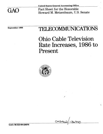
Adjustment Factors for Cable Current Carrying CalculationsUnderground cable ampacity values provided by cable manufacturers or relevantstandards such as the NEC and IEEE Std 835-1994, are frequently based on specificlaying conditions that were considered as important relative to the cable’s immediatesurrounding environment. Site specific conditions can include the following:-Soil thermal resistivity (RHO) of 90 C–cm/W-Installation under an isolated condition-Ambient temperature of 20 C or 40 C-Installation of groups of three or six cable circuitsUsually, conditions in which the cable was installed do not match with those for whichampacities were calculated. This difference can be treated as a medium that isinserted between the base conditions (conditions that were used for calculation by themanufacturer or relevant institutions) and actual site conditions. This approach ispresented in the figure below.Actual conditions ofuseImmediatesurroundingenvironmentbase conditionsAdjustment factor (s)Immediate surrounding environment(Adjustment factors requiered)In principle, specified (base) ampacities need to be adjusted by using correctivefactors to take into account the effect of the various conditions of use. A method forthe calculation of cable ampacities illustrates the concept of cable derating andpresents corrective factors that have effects on cable operating temperatures andhence cable conductor current capacities. In essence, this method uses deratingcorrective factors against base ampacity to provide ampacity relevant to site

conditions. This concept can be summarized as follows:𝐼𝐼 ′ 𝐹𝐹 𝐼𝐼where,𝐼𝐼 ′ is the current carrying capacity under the actual site conditions,𝐹𝐹 is the total cable ampacity correction factor, and𝐼𝐼 is the base current carrying capacity which is usually determined by themanufacturers or relevant industry standards.The overall cable adjustment factor is a correction factor that takes into account thedifferences in the cable’s actual installation and operating conditions from the baseconditions. This factor establishes the maximum load capability that results in anactual cable life equal to or greater than that expected when operated at the baseampacity under the specified conditions. The total cable ampacity correction factor ismade up of several components and can be expressed as:𝐹𝐹 𝐹𝐹𝑡𝑡 𝐹𝐹𝑡𝑡ℎ 𝐹𝐹𝑔𝑔where,𝐹𝐹𝑡𝑡 is the correction factor that accounts for conductor temperature differencesbetween the base case and actual site conditions,𝐹𝐹𝑡𝑡ℎ is the correction factor that accounts for the difference in the soil thermal resistivity,from the 90 C–cm/W at which the base ampacities are specified to the actual soilthermal resistivity, and𝐹𝐹𝑔𝑔 - is the correction factor that accounts for cable derating due to cable grouping.Computer software based on Neher-McGrath method was developed to calculatecorrection factors 𝐹𝐹𝑡𝑡ℎ and 𝐹𝐹𝑔𝑔 . It is used to calculate conductor temperatures for variousinstallation conditions. This procedure considers each correction factor and togetheraccount for the overall derating effects.The aforementioned correction factors are almost completely independent from eachother. Even though specific software can simulate various configurations, the tables

presenting correction factors are based on the following simplified assumptions:-Voltage ratings and cable sizes are used to combine cables for the tablespresenting Fth factors. For specific applications in which RHO is considerablyhigh and mixed group of cables are installed, correlation between correctionfactors cannot be neglected and error can be expected when calculating theoverall conductor temperatures.-Effect of the temperature rise due to the insulation dielectric losses is notconsidered for the temperature adjustment factor Ft. Temperature rise for polyethylene insulated cables rated below 15 kV is less than 2 C. If needed, thiseffect can be considered in Ft by adding the temperature rise due to thedielectric losses to the ambient temperatures 𝑇𝑇 and Ta′ .In situations when high calculation accuracy is needed, previously listed assumptionscannot be neglected. However, cable current carrying capacity obtained using manualmethods can be used as a starting approximation for complex computer solutions thatcan provide actual results based on the real design and cable laying conditions.Ambient and Conductor Temperature Adjustment Factor (Ft)Then ambient and conductor temperature adjustment factor is used to assess theunderground cable ampacity in the case when the cable ambient operatingtemperature and the maximum permissible conductor temperature are different fromthe basic, starting temperature at which the cable base ampacity is defined. Theequations for calculating changes in the conductor and ambient temperatures on thebase cable ampacity are:𝑇𝑇 ′ 𝑇𝑇 ′234.5 𝑇𝑇𝑇𝑇 ′ 𝑇𝑇 ′228.1 𝑇𝑇1/2- Copper1/2- Aluminium𝐹𝐹𝑡𝑡 𝑇𝑇𝑐𝑐 𝑇𝑇𝑎𝑎 234.5 𝑇𝑇𝑐𝑐′ 𝑐𝑐𝑎𝑎𝑐𝑐𝐹𝐹𝑡𝑡 𝑇𝑇𝑐𝑐 𝑇𝑇𝑎𝑎 228.1 𝑇𝑇𝑐𝑐′ 𝑐𝑐𝑎𝑎𝑐𝑐where,Tc is the rated temperature of the conductor in C at which the base cable rating is

specified,Tc′ is the maximum permissible operating temperature in C of the conductor,Ta is the temperature of the ambient temperature in C at which the base cable ratingis defined, andTa′ is the maximum soil ambient temperature in C.It is very difficult to estimate the maximum ambient temperature since it has to bedetermined based on historic data. For installation of underground cables, Ta′ is themaximum soil temperature during summer at the depth at which the cable is buried.Generally, seasonal variations of the soil temperature follow sinusoidal pattern withthe temperature of the soil reaching peak temperatures during summer months. Theeffect of seasonal soil temperature variation decreases with depth. Once a depth of30 feet is reached, the soil temperature remains relatively constant.Soil characteristics such as density, texture and moisture content as well as soilpavement (asphalt, cement) have considerable impact on the temperature of the soil.In order to achieve maximum accuracy, it is preferable to obtain Ta via field tests andmeasurements instead of using approximations that are based on the maximumatmospheric temperature.For cable circuits that are installed in air, Ta is the maximum air temperature duringsummer peak. Due care needs to be taken for cable installations in shade or underdirect sunlight.Typical Ft adjustment factors for conductor temperatures (T 90 C and 75 C) andtemperatures of the ambient (T 20 C for underground installation and 40 C forabove-ground installation) are summarized in the tables below.𝑇𝑇𝑐𝑐′ in 𝑇𝑎𝑎′ in C40450.77 0.671.00 0.931.17 1.111.34 1.29500.550.851.041.24550.390.760.981.19Table 1. Ft factor for various copper conductors (ambient temp. Tc 75 C and Ta 40 C)

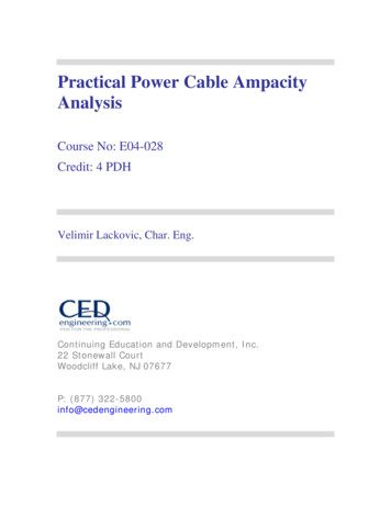
𝑇𝑇𝑐𝑐′ in .191.30𝑇𝑇𝑎𝑎′ in C40450.86 0.790.96 0.901.00 0.951.15 1.111.27 ble 2. Ft factor for various copper conductors, (ambient temp. Tc 90 C and Ta 40 C)𝑇𝑇𝑐𝑐′ in 𝑇𝑎𝑎′ in C20250.87 0.821.00 0.951.10 1.061.21 1.18300.760.901.021.14350.690.850.981.11Table 3. Ft factor for various copper conductors, (ambient temp. Tc 75 C and Ta 20 C)𝑇𝑇𝑐𝑐′ in .131.21𝑇𝑇𝑎𝑎′ in C20250.91 0.870.97 0.931.00 0.961.10 1.061.18 ble 4. Ft factor for various copper conductors, (ambient temp. Tc 90 C and Ta 20 C)Thermal Resistivity Adjustment Factor (Fth)Soil thermal resistivity (RHO) presents the resistance to heat dissipation of the soil. Itis expressed in C–cm/W. Thermal resistivity adjustment factors are presented in thetable below for various underground cable laying configurations in cases in which RHOdiffers from 90 C–cm/W at which the base current carrying capacities are defined. Thepresented tables are based on assumptions that the soil has a uniform and constantthermal resistivity.

RHO ( C-cm/W)Cable Size Number of CKT 60 90 120 140 160 180#12-#111.03 1 0.97 0.96 0.94 0.9331.06 1 0.95 0.92 0.89 0.8761.09 1 0.93 0.89 0.85 0.829 1.11 1 0.92 0.87 0.83 0.791/0-4/011.04 1 0.97 0.95 0.93 0.9131.07 1 0.94 0.9 0.87 0.8561.1 1 0.92 0.87 0.84 0.819 1.12 1 0.91 0.85 0.81 0.78250-100011.05 1 0.96 0.94 0.92 0.931.08 1 0.93 0.89 0.86 0.8361.11 1 0.91 0.86 0.83 0.89 1.13 1 0.9 0.84 0.8 .69Table 4. Fth: Adjustment factor for 0–1000 V cables in duct banks.Base ampacity given at an RHO of 90 C–cm/WCable Size Number of CKT#12-#11369 1/0-4/01369 250-10001369 RHO ( C-cm/W)60 90 120 140 160 180 200 2501.03 1 0.97 0.95 0.93 0.91 0.9 0.881.07 1 0.94 0.90 0.87 0.84 0.81 0.771.09 1 0.92 0.87 0.84 0.80 0.77 0.721.10 1 0.91 0.85 0.81 0.77 0.74 0.691.04 1 0.96 0.94 0.92 0.90 0.88 0.851.08 1 0.93 0.89 0.86 0.83 0.80 0.751.10 1 0.91 0.86 0.82 0.79 0.77 0.711.11 1 0.90 0.84 0.80 0.76 0.73 0.681.05 1 0.95 0.92 0.90 0.88 0.86 0.841.09 1 0.92 0.88 0.85 0.82 0.79 0.741.11 1 0.91 0.85 0.81 0.78 0.75 0.701.12 1 0.90 0.84 0.79 0.75 0.72 0.67Table 5. Fth: Adjustment factor for 1000–35000 V cables in duct banks.Base ampacity given at an RHO of 90 C–cm/W

RHO ( C-cm/W)Cable Size Number of CKT 60 90 120 140 160 180#12-#111.10 1 0.91 0.86 0.82 0.7921.13 1 0.9 0.85 0.81 0.773 1.14 1 0.89 0.84 0.79 0.751/0-4/011.13 1 0.91 0.86 0.81 0.7821.14 1 0.9 0.85 0.8 0.763 1.15 1 0.89 0.84 0.78 0.74250-100011.14 1 0.9 0.85 0.81 0.7821.15 1 0.89 0.84 0.8 0.763 1.15 1 0.88 0.83 0.78 0.70.670.710.690.670.710.690.67Table 6. Fth: Adjustment factor for directly buried cables in duct banks.Base ampacity given at an RHO of 90 C–cm/WSoil thermal resistivity depends on a number of different factors including moisturecontent, soil texture, density, and its structural arrangement. Generally, higher soildensity or moisture content cause better dissipation of heat and lower thermalresistivity. Soil thermal resistivity can have a vast range being less than 40 to morethan 300 C–cm/W. Therefore, a direct soil test is essential especially for criticalapplications. It is important to perform this test after dry peak summer when themoisture content in the soil is minimal. Field tests usually indicate wide ranges of soilthermal resistance for a specific depth. In order to properly calculate cable currentcarrying capacity, the maximum value of the thermal resistivities should be used.Soil dryout effect that is caused by continuously loading underground cables can beconsidered by taking a higher thermal resistivity adjustment factor than the value thatis obtained at site. Special backfill materials such as dense sand can be used to lowerthe effective overall thermal resistivity. These materials can also offset the soil dryouteffect. Soil dryout curves of soil thermal resistivity versus moisture content can be usedto select an appropriate value.Grouping Adjustment Factor (Fg)Cables that are installed in groups operate at higher temperatures than isolatedcables. Operating temperature increases due to the presence of the other cables inthe group which act as heating sources. Therefore, temperature increment caused byproximity of other cable circuits depends on circuit separation and surrounding media(soil, backfilling material, etc.). Generally, increasing the horizontal and vertical

separation between the cables would decrease the temperature interference betweenthem and would consequently increase the value of Fg factor.Fg correlation factors can vary widely depending on the laying conditions. They areusually found in cable manufacturer catalogues and technical specifications. Thesefactors can serve as a starting point for initial approximation and can be later used asan input for a computer program.Computer studies have shown that for duct bank installations, size and voltage ratingof underground cables make a difference in the grouping adjustment factor. Thesefactors are grouped as a function of cable size and voltage rating. In the case differentcables are installed in the same duct bank, the value of the grouping adjustment factoris different for each cable size. In these situations, cable current carrying capacitiescan be determined by calculating cable ampacities starting from the worst (hottest)conduit location to the best (coolest) conduit location. This procedure will allowestablishment of the most economical cable laying arrangement.Other Important Cable Sizing ConsiderationsIn order to achieve maximum utilization of the power cable, reduce operational costs,and minimize capital expanses, an important factor to consider is the proper selectionof the conductor size. In addition, several other factors such as voltage drop, cost oflosses, and the ability to carry short circuit currents should be considered. However,continuous current carrying capacity is of paramount importance.Underground Cable Short Circuit Current CapabilityWhen selecting the short circuit rating of a cable system, several factors are veryimportant and need to be taken into account:-The maximum allowable temperature limit of the cable components (conductor,insulation, metallic sheath or screen, bedding armour, and oversheath). For themajority of the cable systems, endurance of cable dielectric materials are amajor concern and limitation. Energy that produces temperature rise is usuallyexpressed by an equivalent I2t value or the current that flows through theconductor in a specified time interval. Using this approach, the maximum

permitted duration for a given short circuit current value can be properlycalculated.-The maximum allowable value of current that flows through conductor that willnot cause mechanical breakdown due to increased mechanical forces.Regardless of set temperature limitations, this determines a maximum currentwhich must not be exceeded.-The thermal performance of cable joints and terminations at defined currentlimits for the associated cable. Cable accessories also need to withstandmechanical, thermal and electromagnetic forces that are produced by the shortcircuit current in the underground cable.-The impact of the installation mode on the above factors.The first factor is dealt with in more details and the results presented are based onlyon cable considerations. It is important to note that single short circuit currentapplication will not cause any significant damage of the underground cable butrepeated faults may cause cumulative damage which can eventually lead to cablefailure.It is not easy and feasible to determine complete limits for cable terminations and jointsbecause their design and construction are not uniform and standardized, so theirperformance can vary. Therefore cable accessories should be designed and selectedappropriately; however, it is not always financially justifiable and the short-circuitcapability of an underground cable system may not be determined by the performanceof its terminations and joints.Calculation of Permissible Short-Circuit CurrentsShort-circuit ratings can be determined following the adiabatic process methodology,which considers that all heat that is generated remains contained within the currenttransferring component, or non-adiabatic methodology, which considers the fact thatthe heat is absorbed by adjacent materials. The adiabatic methodology can be usedwhen the ratio of the short-circuit duration to the conductor cross-sectional area is less𝑠𝑠than 0.1𝑚𝑚𝑚𝑚2 . For smaller conductors, such as screen wires, loss of heat from the

conductor becomes more important as the short-circuit duration increases. In thoseparticular cases the non-adiabatic methodology can be used to give a considerableincrease in allowable short-circuit currents.Adiabatic method for short circuit current calculationThe adiabatic methodology, that neglects the loss of heat, is correct enough for thecalculation of the maximum allowable short-circuit currents of the conductor andmetallic sheath. It can be used in the majority of practical applications, and

installed. Only power cables need to be considered in this assessment but space needs to be allowed for spare ducts or for control and instrumentation cables. 2. The cable duct needs to be designed considering connected circuits, cable conductor axial separation, space available for the bank and factors that affect cable ampacity.