Transcription
Introduction toStatisticswith GraphPad PrismVersion 2019-11
Introduction to Statistics with GraphPad Prism2LicenceThis manual is 2015-19, Anne Segonds-Pichon.This manual is distributed under the creative commons Attribution-Non-Commercial-Share Alike 2.0licence. This means that you are free: to copy, distribute, display, and perform the work to make derivative worksUnder the following conditions: Attribution. You must give the original author credit. Non-Commercial. You may not use this work for commercial purposes. Share Alike. If you alter, transform, or build upon this work, you may distribute the resultingwork only under a licence identical to this one.Please note that: For any reuse or distribution, you must make clear to others the licence terms of this work.Any of these conditions can be waived if you get permission from the copyright holder.Nothing in this license impairs or restricts the author's moral rights.Full details of this licence can be found /uk/legalcode
Introduction to Statistics with GraphPad Prism3Table of ContentsIntroduction to Statistics with GraphPad Prism . 1Introduction . 5Chapter 1: sample size estimation . 6What is Power? . 6What is Effect Size? . 7Effect size determined by substantive knowledge . 7Effect size determined from previous research . 8Effect size determined by conventions . 8So how is that effect size calculated anyway? . 9Doing power analysis . 10The problem with overpower . 12Sample size (n): biological vs. technical replicates ( repeats) . 13Design 1: As bad as it can get . 14Design 2: Marginally better, but still not good enough . 15Design 3: Often, as good as it can get . 15Design 4: The ideal design . 16Replication at multiple levels . 17Examples of power calculation . 19Comparing 2 proportions . 19Comparing 2 means . 23Unequal sample sizes . 24Power calculation for non-parametric tests . 25Chapter 2: Some key concepts . 26A bit of theory: the null hypothesis and the error types. . 26A bit of theory: Statistical inference . 27The signal-to-noise ratio . 28Chapter 3: Descriptive statistics . 293-1 A bit of theory: descriptive stats . 29The median: . 29The mean . 29The variance . 30The Standard Deviation (SD) . 30Standard Deviation vs. Standard Error . 31Confidence interval . 313-2 A bit of theory: Assumptions of parametric data . 33Chapter 4: Comparing 2 groups . 35How can we check that our data are parametric/normal? . 35Example . 354-1 Power analysis with a t-test . 354-2 Data exploration . 364-3 Student’s t-test . 41A bit of theory . 41Independent t-test . 43Paired t-test . 45Example . 454-4 Non-parametric data. 48Independent groups: Mann-Whitney ( Wilcoxon’s rank-sum) test . 49Example . 49Dependent groups: Wilcoxon’s signed-rank test . 50Example . 51
Introduction to Statistics with GraphPad Prism4Chapter 5: Comparing more than 2 means . 525-1 Comparison of more than 2 means: One-way Analysis of variance . 52A bit of theory . 52Example . 55Power analysis with an ANOVA . 555-2 Non-parametric data: Kruskal-Wallis test . 59Example . 595-3 Two-way Analysis of Variance (File: goggles.xlsx) . 60Example . 615-4 Non-parametric data . 68Chapter 6: Correlation . 69Example . 696-1: Pearson coefficient . 69A bit of theory . 69Power analysis with correlation . 726-2 Linear correlation: goodness-of-fit of the model . 73Example . 736-2 Non-parametric data: Spearman correlation coefficient . 77Example . 77Chapter 7: Curve fitting: Dose-response . 79Example . 81Chapter 8: Qualitative data. 848-1 Comparing 2 groups . 84Example . 84Power Analysis with qualitative data . 84A bit of theory: the Chi2 test . 878-1 Comparing more than 2 groups . 91Example . 91Chapter 9: Survival analysis . 94Time to event and censoring . 94Example of time to event data . 96Example . 96Comparing 2 samples . 99Example . 99Hazard function . 100Comparing more than 2 samples . 101Example . 101References . 104
Introduction to Statistics with GraphPad Prism5IntroductionGraphPad Prism is a straightforward package with a user-friendly environment. There is a lot of easyto-access documentation and the tutorials are very good.Graphical representation of data is pivotal when we want to present scientific results, in particular forpublications. GraphPad allows us to build top quality graphs, much better than Excel for example andin a much more intuitive way.In this manual, however, we are going to focus on the statistical menu of GraphPad. The data analysisapproach is much friendlier than with R for instance. R does not hold your hand all the way through theanalysis, whereas GraphPad does. On the down side, GraphPad is not as powerful as R - as in wecannot do as many as different analyses with GraphPad as we can with R. If we are interested in linearmodelling for example, we would need to use R.Both GraphPad and R work quite differently. Despite this, whichever program we choose we need somebasic statistical knowledge if only to design our experiments correctly, so there is no way out of it!And don’t forget: we use stats to present our data in a comprehensible way and to make our point; thisis just a tool, so don’t hate it, use it!“Forget about getting definitive results from a single experiment; instead embrace variation, acceptuncertainty, and learn what you can." Andrew Gelman, 2018.
Introduction to Statistics with GraphPad Prism6Chapter 1: sample size estimationIt’s practically impossible to collect data on an entire population of interest. Instead we examine datafrom a random sample to provide support for or against our hypothesis. Now the question is: how manysamples/participants/data points should we collect?Power analysis allows us to determine the sample sizes needed to detect statistical effects with highprobability.Experimenters often guard against false positives with statistical significance tests. After an experimenthas been run, we are concerned about falsely concluding that there is an effect when there really isn’t.Power analysis asks the opposite question: supposing there truly is a treatment effect and we were torun our experiment a huge number of times, how often will we get a statistically significant result?Answering this question requires informed guesswork. We’ll have to supply guesses as to how big ourtreatment effect can reasonably be for it to be biologically/clinically relevant/meaningful.What is Power?First, the definition of power: probability that a statistical test will reject a false null hypothesis (H0) whenthe alternative hypothesis (H1) is true. We can also say: it is the probability of detecting a specified effectat a specified significance level. Now ‘specified effect’ refers to the effect size which can be the resultof an experimental manipulation or the strength of a relationship between 2 variables. And this effectsize is ‘specified’ because prior to the power analysis we should have an idea of the size of the effectwe expect to see. The ‘probability of detecting’ bit refers to the ability of a test to detect an effect of aspecified size. The recommended power is 0.8 which means we have an 80% chance of detecting aneffect if one genuinely exists.Power is defined in the context of hypothesis testing. A hypothesis (statistical) test tells us the probabilityof our result (or a more extreme result) occurring, if the null hypothesis is true. If the probability is lowerthan a pre-specified value (alpha, usually 0.05), it is rejected.The null hypothesis (H0) corresponds to the absence of effect and the aim of a statistical test is to rejector not H0. A test or a difference are said to be “significant” if the probability of type I error is: α 0.05(max α 1). It means that the level of uncertainty of a test usually accepted is 5%.Type I error is the incorrect rejection of a true null hypothesis (false positive). Basically, it is theprobability of thinking we have found something when it is not really there.Type II on the other hand, is the failure to reject a false null hypothesis (false negative), so saying thereis nothing going on whereas actually there is. There is a direct relation between Type II error and power,as Power 1 – β where β 0.20 usually hence power 0.8 (probability of drawing a correct conclusionof an effect). We will go back to it in more detail later.Below is a graphical representation of what we have covered so far. H 1 is the alternative hypothesisand the critical value is the value of the difference beyond which that difference is considered significant.
7Introduction to Statistics with GraphPad PrismStatistical decisionTrue state of H0H0 True (no effect)H0 False (effect)Reject H0Type I error (False Positive) αCorrect (True Positive)Do not reject H0Correct (True Negative)Type II error (False Negative) βThe ability to reject the null hypothesis depends upon alpha but also the sample size: a larger samplesize leads to more accurate parameter estimates, which leads to a greater ability to find what we werelooking for. The harder we look, the more likely we are to find it. It also depends on the effect size: thesize of the effect in the population: the bigger it is, the easier it will be to find.What is Effect Size?Power analysis allows us to make sure that we have looked hard enough to find something interesting.The size of the thing we are looking for is the effect size. Several methods exist for deciding what effectsize we would be interested in. Different statistical tests have different effect sizes developed for them,however, the general principle is the same. The first step is to make sure to have preliminary knowledgeof the effect we are after. And there are different ways to go about it.Effect size determined by substantive knowledgeOne way is to identify an effect size that is meaningful i.e. biologically relevant. The estimation of suchan effect is often based on substantive knowledge. Here is a classic example: It is hypothesised that40 year old men who drink more than three cups of coffee per day will score more highly on the CornellMedical Index (CMI: a self-report screening instrument used to obtain a large amount of relevantmedical and psychiatric information) than same-aged men who do not drink coffee. The CMI rangesfrom 0 to 195, and previous research has shown that scores on the CMI increase by about 3.5 pointsfor every decade of life. Therefore, if drinking coffee caused a similar increase in CMI, it would warrantconcern, and so an effect size can be calculated based on that assumption.
8Introduction to Statistics with GraphPad PrismEffect size determined from previous researchAnother approach is to base the estimation of an interesting effect size on previous research, see whateffect sizes other researchers studying similar fields have found. Once identified, it can be used toestimate the sample size.Effect size determined by conventionsYet another approach is to use conventions. Cohen (author of several books and articles on poweranalysis) has defined small, medium and large effect sizes for many types of test. These form usefulconventions, and can guide you if you know approximately how strong the effect is likely to be.Table 1: Thresholds/Convention for interpreting effect sizeTestRelevanteffect sizet-test for meansF-test for ANOVAt-test for correlationChi-square2 proportionsdfrwhSmall0.20.10.10.10.2Effect Size 8Note: The rationale for these benchmarks can be found in Cohen (1988); Rosenthal (1996) later addedthe classification of very large.The graphs below give a visual representation of the effect sizes.Krzywinski and Altman 2013 (Nature Methods)Below is a link to a sliding tool providing a visual approach to Cohen’s effect size:http://rpsychologist.com/d3/cohend/
Introduction to Statistics with GraphPad Prism9The point is sample size is always determined to detect some hypothetical difference. It takes hugesamples to detect tiny differences but tiny samples to detect huge differences, so you have to specifythe size of the effect you are trying to detect.So how is that effect size calculated anyway?Let’s start with an easy example. If we think about comparing 2 means, the effect size, called Cohen’sd, is just the standardised difference between 2 groups:The standard deviation is a measure of the spread of a set of values. Here it refers to the standarddeviation of the population from which the different treatment groups were taken. In practice, however,this is almost never known, so it must be estimated either from the standard deviation of the controlgroup, or from a 'pooled' value from both groups.McGraw and Wong (1992) have suggested a 'Common Language Effect Size' (CLES) statistic, whichthey argue is readily understood by non-statisticians (shown in column 5 of Table 2). This is theprobability that a score sampled at random from one distribution will be greater than a score sampledfrom another. They give the example of the heights of young adult males and females, which differ by
10Introduction to Statistics with GraphPad Prisman effect size of about 2, and translate this difference to a CLES of 0.92. In other words 'in 92 out of100 blind dates among young adults, the male will be taller than the female'.Table 2: Interpretation of Effect Size (Robert Coe, 2002)Percentage ofcontrol groupEffectSizeProbability thatProbability that person fromRank of person in a control you could guessexperimental group will bebelow average group of 25 equivalent towhich group ahigher than person fromperson inthe average person inperson was incontrol, if both chosen atexperimentalexperimental groupfrom knowledgerandom ( CLES)groupof their %2nd0.760.842.098%1st0.840.92Doing power analysisThe main output of a power analysis is the estimation of a sufficient sample size. This is of pivotalimportance of course. If our sample is too big, it is a waste of resources; if it is too small, we may missthe effect (p 0.05) which would also mean a waste of resources. On a more practical point of view,when we write a grant, we need to justify our sample size which we can do through a power analysis.Finally, it is all about the ethics of research, really, which is encapsulated in the UK Home office’s 3 R:Replacement, Refinement and Reduction. The latter in particular relates directly to power calculationas it refers to ‘methods which minimise animal use and enable researchers to obtain comparable levelsof information from fewer animals’ (NC3Rs website).When should we run a power analysis? It depends on what we expect from it: the most common outputbeing the sample size, we should run it before doing the actual experiment (a priori analysis). Thecorrect sequence from hypothesis to results should be:
Introduction to Statistics with GraphPad Prism11HypothesisExperimental designChoice of a Statistical testPower analysisSample sizeExperiment(s)(Stat) analysis of the resultsPractically, the power analysis depends on the relationship between 6 variables: the significance level,the desired power, the difference of biological interest, the standard deviation (together they make upfor the effect size), the alternative hypothesis and the sample size. The significance level is about thep-value (α 0.05), the desired power, as mentioned earlier is usually 80% and we already discussedeffect size.Now the alternative hypothesis is about choosing between one and 2-sided tests ( one and 2-tailedtests). This is both a theoretical and a practical issue and it is worth spending a bit of time reflecting onit as it can help understanding this whole idea of power.We saw before that the bigger the effect size, the bigger the power as in the bigger the probability ofpicking up a difference.Going back to one-tailed vs. 2-tailed tests, often there are two alternatives to H0, and two ways the datacould be different from what we expect given H0, but we are only interested in one of them. This willinfluence the way we calculate p. For example, imagine a test finding out about the length of eels. Wehave 2 groups of eels and for one group, say Group 1, we know the mean and standard deviation, foreels length. We can then ask two different questions. First question: ‘What is the probability of eels inGroup 2 having a different length to the ones in Group 1?’ This is called a two-tailed test, as we’dcalculate p by looking at the area under both ‘tails’ of the normal curve (See graph below).And second question: ‘What is the probability of eels in Group 2 being longer than eels in Group 1?’This is a one-tailed test, as we’d calculate p by looking at the area under only one end of the normalcurve. The one-tailed p is just one half of the two-tailed p-value. In order to use a one-tailed test wemust be only interested in one of two possible cases, and be able specify which in advance.
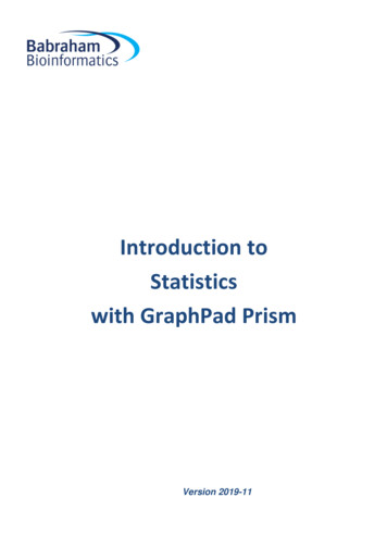
Introduction to Statistics with GraphPad Prism12If you can reasonably predict the direction of an effect, based on a scientific hypothesis, a 1-tailed testis more powerful than a 2-tailed test. However, it is not always rigidly applied so be cautious when 1tailed tests are reported, especially when accompanied by marginally-significant results! And reviewersare usually very suspicious about them.So far we have discussed 5 out of the 6 variables involved in power analysis: the effect size (differenceof biological interest the standard deviation), the significance level, the desired power and thealternative hypothesis. We are left with the variable that we are actually after when we run a poweranalysis: the sample size.To start with, we saw that the sample size is related to power but how does it work? It is best explainedgraphically.The graph below on the left shows what happens with a sample of n 50, the one of the right whathappens with a bigger sample (n 270). The standard deviation of the sampling distribution ( SEM sostandard error of the mean) decreases as N increases. This has the effect of reducing the overlapbetween the H0 and H1 distributions. Since in reality it is difficult to reduce the variability inherent in data,or the contrast between means, the most effective way of improving power is to increase the samplesize.Krzywinski and Altman 2013 (Nature Methods)So the bigger the sample, the bigger the power and the higher the probability to detect the effect sizewe are after.The problem with overpowerAs we saw, power and effect size are linked so that the bigger the power the smaller the effect size thatcan be detected, as in associated with a significant p-value. The problem is that there is such a thingas overpower. Studies or experiments which produce thousand or hundreds of thousands of data, whenstatistically analysed will pretty much always generate very low p-values even when the effect size isminuscule. There is nothing wrong with the stats, what matters here is the interpretation of the results.
Introduction to Statistics with GraphPad Prism13When the sample size is able to detect differences much finer than the expected effect size, a differencethat is correctly statistically distinct is not practically meaningful (and from the perspective of the "enduser" this is effectively a "false positive" even if it's not a statistical one). Beyond the ethical issuesassociated with overpower, it all comes back to the importance of having in mind a meaningful effectsize before running the experiments.Sample size (n): biological vs. technical replicates( repeats)When thinking about sample size, it is very important to consider the difference between technical andbiological replicates. For example, technical replicates involve taking several samples from one tubeand analysing it across multiple conditions. Biological replicates are different samples measured acrossmultiple conditions. When the experimental unit is an animal, it is pretty easy to make the distinctionbetween the 2 types of replicates.To run proper statistical tests so that we can make proper inference from sample to general population,we need biological samples. Staying with mice, if we randomly select one white and one grey mouseand measure their weights, we will not be able to draw any conclusions about whether grey mice are,say, heavier in general. This is because we only have two biological samples.
Introduction to Statistics with GraphPad Prism14If we repeat the meas
Introduction to Statistics with GraphPad Prism 5 Introduction GraphPad Prism is a straightforward package with a user-friendly environment. There is a lot of easy-to-access documentation and the tutorials are very good. Graphical representation of data is pivotal when