Transcription
Advanced High School StatisticsFirst EditionDavid M Diezdavid@openintro.orgChristopher D BarrYale School of Managementchris@openintro.orgMine Çetinkaya-RundelDuke Universitymine@openintro.orgLeah DorazioSan Francisco University High Schoolleah@openintro.org
Copyright 2015 OpenIntro, Inc. First Edition.Printing: July 27th, 2015.This textbook is available under a Creative Commons license. Visit openintro.org for a freePDF, to download the textbook’s source files, or for more information about the license.AP is a trademark registered and owned by the College Board, which was not involved in the production of,and does not endorse, this product.
Contents1 Data collection1.1 Case study . . . . . . . . . . . . . . . . . . .1.2 Data basics . . . . . . . . . . . . . . . . . . .1.3 Overview of data collection principles . . . .1.4 Observational studies and sampling strategies1.5 Experiments . . . . . . . . . . . . . . . . . . .1.6 Exercises . . . . . . . . . . . . . . . . . . . .7810151929342 Summarizing data2.1 Examining numerical data . . . . . . . . .2.2 Numerical summaries and box plots . . .2.3 Considering categorical data . . . . . . . .2.4 Case study: gender discrimination (special2.5 Exercises . . . . . . . . . . . . . . . . . . . . . . . . . . .topic). . . .4545557579843 Probability3.1 Defining probability . .3.2 Conditional probability3.3 The binomial formula .3.4 Simulations . . . . . . .3.5 Random variables . . . .3.6 Continuous distributions3.7 Exercises . . . . . . . .1001001101261321351481514 Distributions of random variables4.1 Normal distribution . . . . . . . . . . . . . .4.2 Sampling distribution of a sample mean . . .4.3 Geometric distribution . . . . . . . . . . . . .4.4 Binomial distribution . . . . . . . . . . . . . .4.5 Sampling distribution of a sample proportion4.6 Exercises . . . . . . . . . . . . . . . . . . . .1641641811901942002035 Foundation for inference5.1 Estimating unknown parameters5.2 Confidence intervals . . . . . . .5.3 Introducing hypothesis testing . .5.4 Does it make sense? . . . . . . .5.5 Exercises . . . . . . . . . . . . .217218219227238240.3.
4CONTENTS6 Inference for categorical data6.1 Inference for a single proportion . . . . . . . . . .6.2 Difference of two proportions . . . . . . . . . . .6.3 Testing for goodness of fit using chi-square . . . .6.4 Homogeneity and independence in two-way tables6.5 Exercises . . . . . . . . . . . . . . . . . . . . . .2512512632732852967 Inference for numerical data7.1 Inference for a single mean with the t-distribution . .7.2 Inference for paired data . . . . . . . . . . . . . . . . .7.3 Difference of two means using the t-distribution . . . .7.4 Comparing many means with ANOVA (special topic) .7.5 Exercises . . . . . . . . . . . . . . . . . . . . . . . . .3113123273353463578 Introduction to linear regression8.1 Line fitting, residuals, and correlation . .8.2 Fitting a line by least squares regression .8.3 Types of outliers in linear regression . . .8.4 Inference for the slope of a regression line8.5 Transformations for nonlinear data . . . .8.6 Exercises . . . . . . . . . . . . . . . . . .374376384394396404407.A End of chapter exercise solutionsB Distribution tablesB.1 Random Number Table . . .B.2 Normal Probability Table . .B.3 t Probability Table . . . . . .B.4 Chi-Square Probability Table.425.447447449452454
PrefaceAdvanced High School Statistics is ready for use with the AP Statistics Course.1This book may be downloaded as a free PDF at openintro.org.We hope readers will take away three ideas from this book in addition to forming a foundation of statistical thinking and methods.(1) Statistics is an applied field with a wide range of practical applications.(2) You don’t have to be a math guru to learn from real, interesting data.(3) Data are messy, and statistical tools are imperfect. But, when you understandthe strengths and weaknesses of these tools, you can use them to learn about thereal world.Textbook overviewThe chapters of this book are as follows:1. Data collection. Data structures, variables, and basic data collection techniques.2. Summarizing data. Data summaries and graphics.3. Probability. The basic principles of probability.4. Distributions of random variables. Introduction to key distributions, and how thenormal model applies to the sample mean and sample proportion.5. Foundation for inference. General ideas for statistical inference in the context ofestimating the population proportion.6. Inference for categorical data. Inference for proportions using the normal and chisquare distributions.7. Inference for numerical data. Inference for one or two sample means using the tdistribution, and comparisons of many means using ANOVA.8. Introduction to linear regression. An introduction to regression with two variables.Instructions are also provided in several sections for using Casio and TI calculators.VideosTheicon indicates that a section or topic has a video overview readily available.The icons are hyperlinked in the textbook PDF, and the videos may also be found atwww.openintro.org/stat/videos.php1 AP is a trademark registered and owned by the College Board, which was not involved in theproduction of, and does not endorse, this product.5
6CONTENTSExamples, exercises, and appendicesExamples and guided practice exercises throughout the textbook may be identified by theirdistinctive bullets:Example 0.1 Large filled bullets signal the start of an example.Full solutions to examples are provided and often include an accompanying table orfigure.JGuided Practice 0.2 Large empty bullets signal to readers that an exercise hasbeen inserted into the text for additional practice and guidance. Students may find ituseful to fill in the bullet after understanding or successfully completing the exercise.Solutions are provided for all within-chapter exercises in footnotes.2There are exercises at the end of each chapter that are useful for practice or homeworkassignments. Many of these questions have multiple parts, and odd-numbered questionsinclude solutions in Appendix A.Probability tables for the normal, t, and chi-square distributions are in Appendix B,and PDF copies of these tables are also available from openintro.org for anyone to download, print, share, or modify.OpenIntro, online resources, and getting involvedOpenIntro is an organization focused on developing free and affordable education materials.OpenIntro Statistics, our first project, is intended for introductory statistics courses at thehigh school through university levels.We encourage anyone learning or teaching statistics to visit openintro.org and getinvolved. We also provide many free online resources, including free course software. Mostdata sets for this textbook are available on the website and through a companion R package.3 OpenIntro’s resources may be used with or without this textbook as a companion.We value your feedback. If there is a particular component of the project you especiallylike or think needs improvement, we want to hear from you. Provide feedback through alink provided on the textbook ementsThis project would not be possible without the dedication and volunteer hours of all thoseinvolved. No one has received any monetary compensation from this project, and we hopeyou will join us in extending a thank you to the project’s volunteers listed atwww.openintro.org/aboutand also to the many students, teachers, and other readers who have provided feedback tothe project.2 Fullsolutions are located down here in the footnote!DM, Barr CD, Çetinkaya-Rundel M. 2015. openintro: OpenIntro data sets and supplementfunctions. github.com/OpenIntroOrg/openintro-r-package.3 Diez
Chapter 1Data collectionScientists seek to answer questions using rigorous methods and careful observations. Theseobservations – collected from the likes of field notes, surveys, and experiments – form thebackbone of a statistical investigation and are called data. Statistics is the study of howbest to collect, analyze, and draw conclusions from data. It is helpful to put statistics inthe context of a general process of investigation:1. Identify a question or problem.2. Collect relevant data on the topic.3. Analyze the data.4. Form a conclusion.Statistics as a subject focuses on making stages 2-4 objective, rigorous, and efficient.That is, statistics has three primary components: How best can we collect data? Howshould it be analyzed? And what can we infer from the analysis?Researchers from a wide array of fields have questions or problems that require thecollection and analysis of data. Let’s consider three examples. Climate scientists: how will the global temperature change over the next 100 years? Psychology: can a simple reminder about saving money cause students to spend less? Political science: what fraction of Americans approve of the job Congress is doing?What questions from current events or from your own life can you think of that could beanswered by collecting and analyzing data? While the questions that can be posed areincredibly diverse, many of these investigations can be addressed with a small number ofdata collection techniques, analytic tools, and fundamental concepts in statistical inference.This chapter focuses on collecting data. We’ll discuss basic properties of data, commonsources of bias that arise during data collection, and several techniques for collecting datathrough both sampling and experiments. After finishing this chapter, you will have thetools for identifying weaknesses and strengths in data-based conclusions, tools that areessential to be an informed citizen and a savvy consumer of information.7
81.1CHAPTER 1. DATA COLLECTIONCase study: using stents to prevent strokesSection 1.1 introduces a classic challenge in statistics: evaluating the efficacy of a medicaltreatment. Terms in this section, and indeed much of this chapter, will all be revisitedlater in the text. The plan for now is simply to get a sense of the role statistics can play inpractice.In this section we will consider an experiment that studies effectiveness of stents intreating patients at risk of stroke.1 Stents are devices put inside blood vessels that assistin patient recovery after cardiac events and reduce the risk of an additional heart attack ordeath. Many doctors have hoped that there would be similar benefits for patients at riskof stroke. We start by writing the principal question the researchers hope to answer:Does the use of stents reduce the risk of stroke?The researchers who asked this question collected data on 451 at-risk patients. Eachvolunteer patient was randomly assigned to one of two groups:Treatment group. Patients in the treatment group received a stent and medicalmanagement. The medical management included medications, management of riskfactors, and help in lifestyle modification.Control group. Patients in the control group received the same medical management as the treatment group, but they did not receive stents.Researchers randomly assigned 224 patients to the treatment group and 227 to the controlgroup. In this study, the control group provides a reference point against which we canmeasure the medical impact of stents in the treatment group.Researchers studied the effect of stents at two time points: 30 days after enrollmentand 365 days after enrollment. The results of 5 patients are summarized in Table 1.1.Patient outcomes are recorded as “stroke” or “no event”, representing whether or not thepatient had a stroke at the end of a time atment.0-30 daysno eventstrokeno event.0-365 daysno eventstrokeno eventcontrolcontrolno eventno eventno eventno eventTable 1.1: Results for five patients from the stent study.Considering data from each patient individually would be a long, cumbersome pathtowards answering the original research question. Instead, performing a statistical dataanalysis allows us to consider all of the data at once. Table 1.2 summarizes the raw data ina more helpful way. In this table, we can quickly see what happened over the entire study.For instance, to identify the number of patients in the treatment group who had a stroke1 Chimowitz MI, Lynn MJ, Derdeyn CP, et al.2011.Stenting versus Aggressive Medical Therapy for Intracranial Arterial Stenosis.New England Journal of Medicine 365:9931003. www.nejm.org/doi/full/10.1056/NEJMoa1105335. NY Times article reporting on the 8stent.html.
1.1. CASE STUDY9within 30 days, we look on the left-side of the table at the intersection of the treatmentand stroke: 33.treatmentcontrolTotal0-30 daysstroke no event3319113214464050-365 daysstroke no event451792819973378Table 1.2: Descriptive statistics for the stent study.JGuided Practice 1.1 What proportion of the patients in the treatment group hadno stroke within the first 30 days of the study? (Please note: answers to all in-textexercises are provided using footnotes.)2We can compute summary statistics from the table. A summary statistic is a singlenumber summarizing a large amount of data.3 For instance, the primary results of thestudy after 1 year could be described by two summary statistics: the proportion of peoplewho had a stroke in the treatment and control groups.Proportion who had a stroke in the treatment (stent) group: 45/224 0.20 20%.Proportion who had a stroke in the control group: 28/227 0.12 12%.These two summary statistics are useful in looking for differences in the groups, and we arein for a surprise: an additional 8% of patients in the treatment group had a stroke! This isimportant for two reasons. First, it is contrary to what doctors expected, which was thatstents would reduce the rate of strokes. Second, it leads to a statistical question: do thedata show a “real” difference between the groups?This second question is subtle. Suppose you flip a coin 100 times. While the chancea coin lands heads in any given coin flip is 50%, we probably won’t observe exactly 50heads. This type of fluctuation is part of almost any type of data generating process. It ispossible that the 8% difference in the stent study is due to this natural variation. However,the larger the difference we observe (for a particular sample size), the less believable it isthat the difference is due to chance. So what we are really asking is the following: is thedifference so large that we should reject the notion that it was due to chance?While we don’t yet have our statistical tools to fully address this question on ourown, we can comprehend the conclusions of the published analysis: there was compellingevidence of harm by stents in this study of stroke patients.Be careful: do not generalize the results of this study to all patients and all stents.This study looked at patients with very specific characteristics who volunteered to be apart of this study and who may not be representative of all stroke patients. In addition,there are many types of stents and this study only considered the self-expanding Wingspanstent (Boston Scientific). However, this study does leave us with an important lesson: weshould keep our eyes open for surprises.2 There were 191 patients in the treatment group that had no stroke in the first 30 days. There were33 191 224 total patients in the treatment group, so the proportion is 191/224 0.85.3 Formally, a summary statistic is a value computed from the data. Some summary statistics are moreuseful than others.
10CHAPTER 1. DATA COLLECTION1.2Data basicsEffective presentation and description of data is a first step in most analyses. This sectionintroduces one structure for organizing data as well as some terminology that will be usedthroughout this book.1.2.1Observations, variables, and data matricesTable 1.3 displays rows 1, 2, 3, and 50 of a data set concerning 50 emails received duringearly 2012. These observations will be referred to as the email50 data set, and they are arandom sample from a larger data set that we will see in Section 2.3.Each row in the table represents a single email or case.4 The columns represent characteristics, called variables, for each of the emails. For example, the first row representsemail 1, which is not spam, contains 21,705 characters, 551 line breaks, is written in HTMLformat, and contains only small numbers.In practice, it is especially important to ask clarifying questions to ensure importantaspects of the data are understood. For instance, it is always important to be sure weknow what each variable means and the units of measurement. Descriptions of all fiveemail variables are given in Table 1.4.123.spamnonoyes.num char21,7057,011631.line ne.50no15,829242htmlsmallTable 1.3: Four rows from the email50 data matrix.variablespamnum charline breaksformatnumberdescriptionSpecifies whether the message was spamThe number of characters in the emailThe number of line breaks in the email (not including text wrapping)Indicates if the email contained special formatting, such as bolding, tables,or links, which would indicate the message is in HTML formatIndicates whether the email contained no number, a small number (under1 million), or a large numberTable 1.4: Variables and their descriptions for the email50 data set.The data in Table 1.3 represent a data matrix, which is a common way to organizedata. Each row of a data matrix corresponds to a unique case, and each column correspondsto a variable. A data matrix for the stroke study introduced in Section 1.1 is shown inTable 1.1 on page 8, where the cases were patients and there were three variables recordedfor each patient.Data matrices are a convenient way to record and store data. If another individualor case is added to the data set, an additional row can be easily added. Similarly, anothercolumn can be added for a new variable.4Acase is also sometimes called a unit of observation or an observational unit.
1.2. DATA BASICS11all inalordinal(unordered categorical)(ordered categorical)Figure 1.5: Breakdown of variables into their respective types.JGuided Practice 1.2 We consider a publicly available data set that summarizesinformation about the 3,143 counties in the United States, and we call this the countydata set. This data set includes information about each county: its name, the statewhere it resides, its population in 2000 and 2010, per capita federal spending, povertyrate, and five additional characteristics. How might these data be organized in a datamatrix? Reminder: look in the footnotes for answers to in-text exercises.5Seven rows of the county data set are shown in Table 1.6, and the variables are summarizedin Table 1.7. These data were collected from the US Census website.61.2.2Types of variablesExamine the fed spend, pop2010, state, and smoking ban variables in the county dataset. Each of these variables is inherently different from the other three yet many of themshare certain characteristics.First consider fed spend, which is said to be a numerical variable since it can takea wide range of numerical values, and it is sensible to add, subtract, or take averages withthose values. On the other hand, we would not classify a variable reporting telephone areacodes as numerical since their average, sum, and difference have no clear meaning.The pop2010 variable is also numerical, although it seems to be a little differentthan fed spend. This variable of the population count can only take whole non-negativenumbers (0, 1, 2, .). For this reason, the population variable is said to be discrete sinceit can only take numerical values with jumps. On the other hand, the federal spendingvariable is said to be continuous.The variable state can take up to 51 values after accounting for Washington, DC: AL,., and WY. Because the responses themselves are categories, state is called a categoricalvariable,7 and the possible values are called the variable’s levels.Finally, consider the smoking ban variable, which describes the type of county-widesmoking ban and takes values none, partial, or comprehensive in each county. Thisvariable seems to be a hybrid: it is a categorical variable but the levels have a naturalordering. A variable with these properties is called an ordinal variable. To simplifyanalyses, any ordinal variables in this book will be treated as categorical variables.5 Eachcounty may be viewed as a case, and there are eleven pieces of information recorded for eachcase. A table with 3,143 rows and 11 columns could hold these data, where each row represents a countyand each column represents a particular piece of information.6 quickfacts.census.gov/qfd/index.html7 Sometimes also called a nominal variable.
896644fed 5income2456826469158751991821070.2855728463med ionCounty nameState where the county resides (also including the District of Columbia)Population in 2000Population in 2010Federal spending per capitaPercent of the population in povertyPercent of the population that lives in their own home or lives with the owner(e.g. children living with parents who own the home)Percent of living units that are in multi-unit structures (e.g. apartments)Income per capitaMedian household income for the county, where a household’s income equalsthe total income of its occupants who are 15 years or olderType of county-wide smoking ban in place at the end of 2011, which takes oneof three values: none, partial, or comprehensive, where a comprehensiveban means smoking was not permitted in restaurants, bars, or workplaces, andpartial means smoking was banned in at least one of those three locationsTable 1.6: Seven rows from the county data e 1.7: Variables and their descriptions for the county data set.smoking banmultiunitincomemed incomevariablenamestatepop2000pop2010fed ng bannonenonenonenonenone.nonenone12CHAPTER 1. DATA COLLECTION
1.2. DATA BASICS13Example 1.3 Data were collected about students in a statistics course. Threevariables were recorded for each student: number of siblings, student height, andwhether the student had previously taken a statistics course. Classify each of thevariables as continuous numerical, discrete numerical, or categorical.The number of siblings and student height represent numerical variables. Becausethe number of siblings is a count, it is discrete. Height varies continuously, so it is acontinuous numerical variable. The last variable classifies students into two categories– those who have and those who have not taken a statistics course – which makesthis variable categorical.JGuided Practice 1.4 Consider the variables group and outcome (at 30 days) fromthe stent study in Section 1.1. Are these numerical or categorical variables?81.2.3Relationships between variablesMany analyses are motivated by a researcher looking for a relationship between two ormore variables. A social scientist may like to answer some of the following questions:(1) Is federal spending, on average, higher or lower in counties with high rates of poverty?(2) If homeownership is lower than the national average in one county, will the percentof multi-unit structures in that county likely be above or below the national average?(3) Which counties have a higher average income: those that enact one or more smokingbans or those that do not?To answer these questions, data must be collected, such as the county data set shownin Table 1.6. Examining summary statistics could provide insights for each of the threequestions about counties. Additionally, graphs can be used to visually summarize data andare useful for answering such questions as well.Scatterplots are one type of graph used to study the relationship between two numerical variables. Figure 1.8 compares the variables fed spend and poverty. Each pointon the plot represents a single county. For instance, the highlighted dot corresponds toCounty 1088 in the county data set: Owsley County, Kentucky, which had a poverty rateof 41.5% and federal spending of 21.50 per capita. The scatterplot suggests a relationshipbetween the two variables: counties with a high poverty rate also tend to have slightly morefederal spending. We might brainstorm as to why this relationship exists and investigateeach idea to determine which is the most reasonable explanation.JGuided Practice 1.5 Examine the variables in the email50 data set, which aredescribed in Table 1.4 on page 10. Create two questions about the relationshipsbetween these variables that are of interest to you.9The fed spend and poverty variables are said to be associated because the plot showsa discernible pattern. When two variables show some connection with one another, they arecalled associated variables. Associated variables can also be called dependent variablesand vice-versa.8 Thereare only two possible values for each variable, and in both cases they describe categories. Thus,each is a categorical variable.9 Two sample questions: (1) Intuition suggests that if there are many line breaks in an email then therewould also tend to be many characters: does this hold true? (2) Is there a connection between whether anemail format is plain text (versus HTML) and whether it is a spam message?
14CHAPTER 1. DATA COLLECTIONFederal Spending Per Capita3032 counties with higherfederal spending are not shown 2010001020304050Poverty Rate (Percent)Figure 1.8: A scatterplot showing fed spend against poverty. OwsleyCounty of Kentucky, with a poverty rate of 41.5% and federal spending of 21.50 per capita, is highlighted.Example 1.6 The relationship between the homeownership rate and the percent ofunits in multi-unit structures (e.g. apartments, condos) is visualized using a scatterplot in Figure 1.9. Are these variables associated?It appears that the larger the fraction of units in multi-unit structures, the lower thehomeownership rate. Since there is some relationship between the variables, they areassociated.Because there is a downward trend in Figure 1.9 – counties with more units in multiunit structures are associated with lower homeownership – these variables are said to benegatively associated. A positive association is shown in the relationship betweenthe poverty and fed spend variables represented in Figure 1.8, where counties with higherpoverty rates tend to receive more federal spending per capita.If two variables are not associated, then they are said to be independent. That is,two variables are independent if there is no evident relationship between the two.Associated or independent, not bothA pair of variables are either related in some way (associated) or not (independent).No pair of variables is both associated and independent.
Percent of Homeownership1.3. OVERVIEW OF DATA COLLECTION t of Units in Multi Unit StructuresFigure 1.9: A scatterplot of homeownership versus the percent of unitsthat are in multi-unit structures for all 3,143 counties. Interested readersmay find an image of this plot with an additional third variable, countypopulation, presented at www.openintro.org/stat/down/MHP.png.1.3Overview of data collection principlesThe first step in conducting research is to identify topics or questions that are to be investigated. A clearly laid out research question is helpful in identifying what subjects or casesshould be studied and what variables are important. It is also important to consider howdata are collected so that they are reliable and help achieve the research goals.1.3.1Populations and samplesConsider the following three research questions:1. What is the average mercury content in swordfish in the Atlantic Ocean?2. Over the last 5 years, what is the average time to complete a degree for Duke undergraduate students?3. Does a new drug reduce the number of deaths in patients with severe heart disease?Each research question refers to a target population. In the first question, the targetpopulation is all swordfish in the Atlantic ocean, and each fish represents a case. Oftentimes, it is too expensive to collect data for every case in a population. Instead, a sampleis taken. A sample represents a subset of the cases and is often a small fraction of thepopulation. For instance, 60 swordfish (or some other number) in the population mightbe selected, and this sample data may be used to provide an estimate of the populationaverage and answer the research question.JGuided Practice 1.7 For the second and third questions above, identify the targetpopulation and what re
Advanced High School Statistics is ready for use with the AP Statistics Course.1 This book may be downloaded as a free PDF at openintro.org. We hope readers will take away three ideas from this book in addition to forming a foun-dation of statistical thinking and methods. (1)Statistics