Transcription
DEPTH FROM ACCIDENTAL MOTION USING GEOMETRY PRIORSung-Hoon Im, Gyeongmin Choe, Hae-Gon Jeon, In So KweonRobotics and Computer Vision Lab, KAIST, KoreaABSTRACTWe present a method to reconstruct dense 3D points fromsmall camera motion. We begin with estimating sparse 3Dpoints and camera poses by Structure from Motion (SfM)method with homography decomposition. Although the estimated points are optimized via bundle adjustment and givesreliable accuracy, the reconstructed points are sparse becauseit heavily depends on the extracted features of a scene. Tohandle this, we propose a depth propagation method usingboth a color prior from the images and a geometry prior fromthe initial points. The major benefit of our method is that wecan easily handle the regions with similar colors but differentdepths by using the surface normal estimated from the initialpoints. We design our depth propagation framework into thecost minimization process. The cost function is linearly designed, which makes our optimization tractable. We demonstrate the effectiveness of our approach by comparing with aconventional method using various real-world examples.Index Terms— Structure from motion, Small baseline,Depth propagation1. INTRODUCTIONEstimating a depth map from multiview images is a majorproblem in the computer vision field since the depth mapplays an important role in many applications such as sceneunderstanding and photographic editing. The most representative approach is SfM [1] which estimates 3D points andcamera poses at the same time. Moreover, bundle adjustment [2] optimizes both the 3D points and camera poses accurately. Although the solution is theoretically optimal, whenthe camera baseline is too small, the metric depth error increases quadratically even with small errors in disparity [3].Various attempts in computational photography have beenmade to measure depth information of a scene without camera motion. In [4, 5, 6], modifications of camera apertures forrobust depth from defocusing were proposed as an alternativeway to compute depth maps. Another approach is by lightfield photography which uses an angular and spatial information of incoming light ray in an image domain. This allowsto obtain multi-view images of a scene in a single shot [7, 8],and the multi-view images are used for depth map estimation [9, 10, 11]. Although these recent progresses of computational photography show alternative ways to compute depth978-1-4799-8339-1/15/ 31.00 2015 IEEE4160(a)(b)(c)(d)Fig. 1: Result comparison. (a) Depth map by [12]. (b) 3Dpoint cloud from (a). (c) Our depth map. (d) 3D point cloudfrom (c).map, they are not available in practice because they requireeither camera modification or loss of image resolution.Recently, Yu and Gallup [12] show that 3D points can bereconstructed from multiple views via an accidental motioncaused by hand shaking or heart beating. It has the potentialto overcome the limitations of coded aperture and light-fieldby capturing a short video without large movement. Since thebaseline between consecutive image sequences is narrow, thecamera poses at each view can be initialized as identical andcan be used for the bundle adjustment. Although the underlying assumption is reasonable, the depth map and 3D pointcloud in Fig. 1-(a), (b) show inaccuracy in the results becauseof unreliable sparse 3D points, which is unsatisfactory for thehigh-quality 3D modeling.In this paper, we target to obtain an accurate 3D pointcloud as well as a depth map from small motion. First, weuse SfM to estimate initial sparse 3D points and camera posesfrom the small motion. In contrast to [12], our method provides a good initial solution of the camera poses by homography decomposition for accurate sparse 3d reconstruction.For dense 3D reconstruction, we propose a depth propagationmethod using both a color prior from the images and a geometry prior from the initial points while the conventional propagation method [13] uses only a color prior. Our depth propagation is designed into the linear cost minimization framework, which effectively improves the depth quality as shownin Fig. 1-(c), (d).ICIP 2015
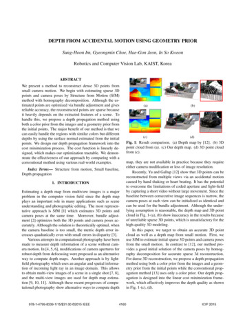
Dataset[12]Proposed(a)Stone (Fig. 1)0.0380.003Wall (Fig. 4)0.3080.094Shop (Fig. 5)0.7490.072Table 1: Initial average reprojection errors comparison between the conventional [12] and proposed initial camera poses(Unit : pixel).(b)Fig. 2: Feature handling. (a) Features on moving objects. (b)Feature removal - Stone [12] : 1920 10802. PROPOSED METHODIn this section, we describe our overall dense 3D reconstruction framework for tiny baseline images. Our system is similar to the 3D reconstruction from accidental motion proposedin [12]. The overall procedure consists of feature extraction,initial sparse 3D reconstruction, and dense 3D reconstruction.We improve the performance in every step on [12], and depthpropagation in Section 2.2 which is the most significant improvement in this paper.2.1. Structure from small motionThis section describes the way to extract reliable features andreconstruct 3D points for small motion precisely. The keyobservation is homography between reference view and theother views.Feature extraction It is important to extract and match features precisely for narrow baseline multiview. If there aresome unreliable feature matchings and features on movingobjects, it causes significant error and should be removed.[12] tracked corner features by Kanade-Lucas-Tomasi (KLT)tracker [14] and removed feature outlier by maximum colorgradient difference. It can only handle features with high localization error, but not features on moving objects. We filterout the features on moving objects by RANSAC [15] for thehomography as shown in Fig. 2. Homography H for eachimage is computed by matched feature points and homography outliers can be detected by RANSAC. If the features areclassified as outliers more than m times, we regard them asfeatures on moving objects.Sparse 3D reconstruction The key idea of 3D reconstruction from small motion is to directly apply bundle adjustmentwith approximated initial depth and camera poses. [12] assumed that the identity matrix for rotation matrix R, zerotranslation T , and randomly assigned depth for initial depth dare good initializations for bundle adjustment input. However,the initial parameters are rough approximations that they arenot suitable for our purpose which is computing reliable 3Dpoints. We propose to set initial camera poses as the decomposition of homography [16]. Homography H is composedas:RT T nT)K 1 ,(1)H K(RT d4161where K and n are camera intrinsic parameter and surfacenormal. Even though the decomposed rotation matrix R andtranslation matrix T with unknown normal vector n and depthd are not precise camera poses, they reduce initial reprojection error leading to well refined camera poses and 3D points.Thus decomposed camera poses can be reliable initial camera poses for bundle adjustment. Table 1. represents the initial projection error comparison between rough initial cameraposes and decomposed initial camera poses. Initial reprojection errors of our initial camera poses are less than that of theconventional method, and more accurate sparse points can beobtained.With reliable initial parameters, bundle adjustment successfully refine depth and camera poses. The cost functionof bundle adjustment is the L2 norm of the reprojection errordefined as:F NFNI XX pij π(K(Ri Pj Ti )) 2 ,(2)i 1 j 1where NI and NF are the number of images and features.Matrix Ri and Ti are camera rotation and translation for eachview point i. World coordinates Pj dj [x1j , y1j , 1] for eachfeature point j are the depth dj multiplication with normalized image coordinates pij [xij , yij ] of reference view. Thefunction π : R3 R2 is the projection function from 3D to2D coordinates. The cost function in Eq. (2) is optimized withLevenberg marquardt (LM) algorithm [17].2.2. Depth propagationThis subsection describes a method to propagate the sparsedepth points initially estimated in Sec. 2.1 into dense depth.Generally, depth propagation using a color cue [18, 19, 13] isfrequently used, but there are many cases where crucial artifacts can occur, especially, in the region where neighboringpixels with similar color have different depth. To handle thisunreliability, we propose a novel optimization method. Wedesign our propagation method minimizing cost function defined as:E(D) Ec (D) λEg (D),(3)where D is the optimal depth. Ec and Eg are color and geometry terms with regularization parameter λ.Color consistency A color consistency term is designedbased on [13] . We assume that the scene depth field is always piecewise smooth. The main idea is that a similar depth
Algorithm 1 Normal vector estimation(a)(b)(c)(d)Nd The number of adjacent sparse control points withina 3D sphere with the radius rdif Nd 2 thenSkip to calculate normal vectorselseCompute normal vectors {n} by plane fitting[U, D, V ] svd(n0 n)Refined normal vectors First column of Uend ifNormal vector propagation by color energy functionFig. 3: Normal vector estimation. (a) Reference image withfeatures. (b) Sparse 3D reconstruction. (c) Sparse normalvectors. (d) Normal map.where Ng is the number of sparse control points within localwindow lw and γg controls the strength of similarity measure.It measures how much the normal vectors of p and q are correlated.value tends to be assigned to an adjacent pixel with high coloraffinity. The cost function for color is defined as: 2X XcEc (D) Dp wpq Dq ,(4)Linear equation Our cost minimization is efficiently solvedby the linear equations Ax b. To find the optimal solutionof the color energy function, we solve OEc (D) 0 which isdefined as:OEc (D) (I W c )D,(8)p Irefq N8 (p)where q is the 8 neighbors of p which belong to pixels incthe reference image Iref . The color similarity weight wpqbetween pixel p and q in lab color space is defined as Iplab Iqlab 1cexp,(5)wpq Ncγcwhere Nc is the normalization factor which makes the sum ofcequal to one and γc is the strength param8-neighboring wpqeter for similarity measure which is manually tuned.Geometric consistency We assume that a normal vector atpoint p is perpendicular to vectors from point p to adjacentsparse control points q on the same plane. The geometry termEg is defined as the sum of the inner products between normal vector at point p and vectors pointing to adjacent sparsecontrol points q.XXgEg (D) wpq np · (Dp Xp Dq Xq )) , (6)p Iref q Gw (p)where q is the set of sparse control points Gw (p) at the center p within the 2D local window lw . The normalized imagecoordinate Xp and the normal vector np are represented by[xp , yp , 1] and [ap , bp , cp ] at the pixel p, respectively. Normalvector np is computed by plane fitting in advance. A planecan be fit using adjacent sparse control points in 3D space andthe fitted plane estimates the adjacent normal vectors. Algorithm 1. shows the normal vector estimation step. To ensuresparse points q are on the same plane with point p, the normalgsimilarity measure wpqbetween points p and q is defined as 1 (1 np · nq )gwpq exp,(7)Ngγg4162where I is the M M matrix (M is the number of pixels)c) matrix. D is aand W c is the pairwise color similarity (wpqone dimensional vector that we optimize.For the geometry energy function, we derive from (6),XXgwpqDp spq 0,(9)p Iref q Gw (p)gwhere spq wpqDqap xq bp yq cp.ap xp bp yp cp(10)and we obtain matrix form as:W g D S 0,(11)gwhere W g is the M M the pairwise normal similarity (wpq)matrix and S is the pairwise element of spq .Both terms are combined with a regularization term λ : I(p, q)p G;At (p, q) (12)((I W c ) λW g )(p, q) p / G. Gp p G;bt (p) (13)λSp p / G.3. EXPERIMENTAL RESULTSThe proposed algorithm is carried out with the parameters asfollows. We set both strength of similarity measure γc and γgas 0.01 and use 49 49 support window lw . The radius rdis calculated by dividing the initial depth over 20. To evaluate the performance of the proposed algorithm, we conduct
(a)(b)(c)(d)Fig. 4: Experiment Result - Wall [12] : 1920 1080. (a) Depth map. (b) Overall 3D point cloud. (c) Enlarged box of (b). (d)Mesh without texture mapping; First row : Yu and Gallup [12], Second row : conventional propagation, Third row : proposedpropagation.(a)(b)(c)(d)(e)Fig. 5: Result of own dataset - Shop : 1296 728. (a) Reference image. (b) Depth map. (c) Mesh with texture mapping. (d)Enlarged box of (c). (d) Mesh without texture mapping.experiments using datasets provided by the author1 (Fig. 1-4)and our own dataset (Fig. 5). To verify the effectiveness of ourinitial camera pose estimation, we compare our result with theresults obtained from [12] and they are shown in the 1st and3rd rows of Fig. 4. As expected, our dense reconstructionresult has less artifacts and more sense of reality. Furthermore, we compare our novel depth propagation method withthe conventional method shown in the 2nd and 3rd rows ofFig. 4, respectively. We show detailed 3D point cloud andmesh in Fig. 4(c)-(d). While the conventional depth propagation method makes a lot of discontinuity across the bricks,the proposed method continuously propagates the depth values, which reconstructs the overall 3D points more reliably.Fig. 5 is the result from our own dataset taken by Cannon EOS60D. We take 90 frames for 3 seconds with less than10mm translation. The depth range of our dataset is from 1mto 10m. As shown in Fig. 5(b)-(c), the overall depth rangeis accurately reconstructed with our method. The details ofthe 3D model are represented in Fig. 5(d)-(e). Supplemen1 http://yf.io/p/tiny/4163tary video and high-resolution results of various outdoor andindoor scenes are available online.4. CONCLUSION AND DISCUSSIONWe have presented a novel method to reconstruct initial sparse3D points and propagate them into dense 3D structure undernarrow-baseline, multi-view imaging setup. By using featureswith less localization errors and more reliable initial cameraposes, more accurate sparse 3D points were obtained. Furthermore, we were able to achieve better dense 3D points bysolving simple linear equations. In the future, we will try toimprove our method robust to motion and depth range by using additional sensors in a cell-phone or DSLR, such as gyrosensor.5. ACKNOWLEDGEMENTThis research is supported by the Study on Imaging Systemsfor the next generation cameras funded by the Samsung Electronics Co., Ltd (DMC R&D center) (IO130806-00717-02).
6. REFERENCES[1] Richard Hartley and Andrew Zisserman, Multiple viewgeometry in computer vision, Cambridge universitypress, 2003.[2] Bill Triggs, Philip F McLauchlan, Richard I Hartley, andAndrew W Fitzgibbon, “Bundle adjustmenta modernsynthesis,” in Vision algorithms: theory and practice,pp. 298–372. Springer, 2000.[3] David Gallup, J-M Frahm, Philippos Mordohai, andMarc Pollefeys, “Variable baseline/resolution stereo,”in Proc. of Computer Vision and Pattern Recognition(CVPR), 2008.[4] Changyin Zhou, Stephen Lin, and Shree K Nayar,“Coded aperture pairs for depth from defocus and defocus deblurring,” Int’l Journal of Computer Vision, vol.93, no. 1, pp. 53–72, 2011.[5] Paul Green, Wenyang Sun, Wojciech Matusik, andFrédo Durand, “Multi-aperture photography,” ACMTrans. on Graph., vol. 26, no. 3, pp. 68, 2007.[6] Ayan Chakrabarti and Todd Zickler, “Depth and deblurring from a spectrally-varying depth-of-field,” in Proc.of European Conf. on Computer Vision (ECCV). 2012,Springer.[7] Ren Ng, Marc Levoy, Mathieu Brédif, Gene Duval,Mark Horowitz, and Pat Hanrahan, “Light field photography with a hand-held plenoptic camera,” StanfordUniversity Computer Science Technical Report CSTR,vol. 2, no. 11, 2005.[8] Andrew Lumsdaine and Todor Georgiev, “The focusedplenoptic camera,” IEEE, 2009.[9] Sven Wanner and Bastian Goldluecke, “Globally consistent depth labeling of 4d light fields,” in Proc.of Computer Vision and Pattern Recognition (CVPR).IEEE, 2012.[10] Michael W Tao, Sunil Hadap, Jitendra Malik, and RaviRamamoorthi, “Depth from combining defocus and correspondence using light-field cameras,” in Proc. of Int’lConf. on Computer Vision (ICCV), 2013, pp. 673–680.[11] Hae-Gon Jeon, Jaesik Park, Gyeongmin Choe, JinsunPark, Yunsu Bok, Yu-Wing Tai, and In So Kweon, “Accurate depth map estimation from a lenslet light fieldcamera,” in Proc. of Computer Vision and PatternRecognition (CVPR), 2015.[12] Fisher Yu and David Gallup, “3d reconstruction fromaccidental motion,” in Proc. of Computer Vision andPattern Recognition (CVPR). IEEE, 2014.4164[13] Liang Wang and Ruigang Yang, “Global stereo matching leveraged by sparse ground control points,” in Proc.of Computer Vision and Pattern Recognition (CVPR),2011.[14] Carlo Tomasi and Takeo Kanade, Detection and tracking of point features, School of Computer Science,Carnegie Mellon Univ. Pittsburgh, 1991.[15] Martin A Fischler and Robert C Bolles, “Random sample consensus: a paradigm for model fitting with applications to image analysis and automated cartography,”Communications of the ACM, vol. 24, no. 6, pp. 381–395, 1981.[16] Yi Ma, An invitation to 3-d vision: from images to geometric models, vol. 26, springer, 2004.[17] Jorge J Moré, The Levenberg-Marquardt algorithm: implementation and theory, Springer, 1978.[18] J. Park, H. Kim, Y.-W. Tai, M. S. Brown, and I. S.Kweon, “High quality depth map upsampling for 3dtof cameras,” in Proc. of Int’l Conf. on Computer Vision(ICCV), 2011.[19] G. Choe, J. Park, Y.-W. Tai, and I.S. Kweon, “Exploiting shading cues in kinect ir images for geometry refinement,” in Proc. of Computer Vision and Pattern Recognition (CVPR), 2014.
tion of incoming light ray in an image domain. This allows to obtain multi-view images of a scene in a single shot [7, 8], and the multi-view images are used for depth map estima-tion [9, 10, 11]. Although these recent progresses of compu-tational photography show alternative ways to