Transcription
Notes on Econometrics IGrace McCormackApril 28, 2019Contents1Overview1.1 Introduction to a general econometrician framework . . . . . . . . . . . . . . . . . . . . . . . . . . . . . . . . . . .1.2 A rough taxonomy of econometric analyses . . . . . . . . . . . . . . . . . . . . . . . . . . . . . . . . . . . . . . .223IProbability & Statistics42Probability2.1 Moment Generating Functions . . . . . . . . . . . . . . . . . . . . . . . . . . . . . . . . . . . . . . . . . . . . . .2.2 Convolutions . . . . . . . . . . . . . . . . . . . . . . . . . . . . . . . . . . . . . . . . . . . . . . . . . . . . . . .5683Bayesian statistics3.1 Bayesian vs. Classical Statistics . . . . . . . . . . . . . . . . . . . . . . . . . . . . . . . . . . . . . . . . . . . . .3.2 Bayesian updating and conjugate prior distributions . . . . . . . . . . . . . . . . . . . . . . . . . . . . . . . . . . .3.3 Decision theory . . . . . . . . . . . . . . . . . . . . . . . . . . . . . . . . . . . . . . . . . . . . . . . . . . . . . .111112144Classical statistics4.1 Estimators . . . . . . . . . . . . . . .4.2 Hypothesis testing . . . . . . . . . . .4.2.1 The Neyman Pearson Lemma4.3 Confidence Intervals . . . . . . . . .4.4 Statistical power and MDE . . . . . .4.5 Chi-Squared Tests . . . . . . . . . . .15161718232427II5.Econometrics29Linear regression5.1 OLS . . . . . . . . . . . . . . . . . . . . . . . .5.2 Confidence intervals . . . . . . . . . . . . . . .5.3 Variance-Covariance Matrix of OLS Coefficients5.4 Gauss-Markov and BLUE OLS . . . . . . . . . .5.5 Heteroskedasticity . . . . . . . . . . . . . . . . .5.6 Weighted Least Squares . . . . . . . . . . . . . .30313437383942Maximum Likelihood Estimation6.1 General MLE framework . . .6.2 Logit and Probit . . . . . . . .6.2.1 Binary Logit . . . . .6.2.2 Binary Probit . . . . .4344484950A Additional ResourcesA.1 General notes . . . . . . . . . . . . . . . . . . . . . . . . . . . . . . . . . . . . . . . . . . . . . . . . . . . . . . .A.2 Notes on specific topics . . . . . . . . . . . . . . . . . . . . . . . . . . . . . . . . . . . . . . . . . . . . . . . . . .5151516.1
21OverviewThis set of notes is intended to supplement the typical first semester of econometrics taken by PhD students in public policy, economics, and other related fields. It was developed specifically for the first year econometrics sequence at the Harvard Kennedy Schoolof Govenrment, which is designed to provide students with tools necessary for economics and political science research related topolicy design. In this vein, I wish us to think of econometrics as a means of using data to understand something about the true natureof the world. The organizing framework for these notes can be seen below. I will be returning to this framework throughout the notes.1.1Introduction to a general econometrician framework1.) We start with a Population Relationship or Population DataGenerating Process (DGP), which we can think about as some“law of nature” that is true about the world. The DGP is definedby some population parameter θ. parameter - a population value or characteristic of the DataGenerating-Process, for example, the mean a distribution orsomeone’s marginal utility of consumption. In this set ofnotes, I will often use θ to denote a population parameter.The population parameter is what generates data and is whatwe want to estimate using statistics or econometricsThe DGP can be something simple, like the density of a normaldistribution in which case θ might be the mean and standarddeviation of the distribution. It could also be something quitecomplicated like the causal effect of education on income, inwhich case θ might be the financial return to each additional yearof education.1.) Population Relationshipor Population Data-Generating Process:yi g(xi θ)where g(·) is just an arbitrary functionand θ is some population parameter.sampling2.) Observe data from a sampleof N observations of i 1 . N{yi , x1i , x2i } i 1.Nestimating2.) This DGP will produce some data from which we willbe able to observe a sample of N observations. For example, ifthe DGP is the normal distribution, we could have a sample of Nnormally distributed variables. If the DGP is the causal effect ofeducation on income, we could have a sample of N people withinformation on incomes and education.3.) We wish to use our data to understand the true population parameter θ. We can characterize the parameter a myriad ofways depending on the context: posterior distribution - the probability distribution of theparameter θ based on the data that we observed (y, x) andsome prior belief of the distribution of the parameter f (θ).This is what we will learn to be called a Bayesian approach. hypothesis test - we can use our data to see if we can rejectvarious hypothesis about our data (for example, a hypothesismay be that the mean of a distribution is 7 or that educationhas no effect on income) estimator - our “best guess” of what the population parameter value is, for example a sample mean or an estimatedOLS coefficient. In this set of notes, I will use a “ˆ” to denote an estimator. While the estimator will often be a singlevalue (a so-called “point estimate”), we also typically haveto characterize how certain we are that this estimator accurately captures the population parameter, typically with aconfidence interval.We will return to this framework more throughout these notes.3.) Characterize parameters of modelusing some econometric method
1.2A rough taxonomy of econometric analyses1.23A rough taxonomy of econometric analysesBefore we get started on the nitty gritties, I would like to take a moment to note how different types of econometric analyses fitbroadly into this framework. Unlike microeconomics, which is taught rather similarly across most first year PhD programs, there issome degree of variation in the typical econometric sequence. You might be uncertain about what type of econometric tools that youshould be learning or exactly what your choice set is to begin with. I will categorize three broad areas that most econometric courseswill fall into (note that this list is not a universally acknowledged taxonomy, but I find it a useful heuristic):1. Reduced form estimation – This is the type of econometrics that is most often used for Labor Economics and Public Economics. This approach entails linear regression to recover some causal effect of X on Y. It is also usef for “sufficient statistics”approaches. This is likely the type of econometrics that you encountered in your undergraduate courses.2. Structural estimation – This type of econometrics is much more common in Industrial Organization. This approach requiresexplicit modeling of the utility function or production function to recover parameters like an individual’s price elasticity orrisk aversion or a firm’s marginal cost of production. In our framework above, we can think of it as requiring the g(xi θ)to be a utility function or some “micro-founded” data-generating process. While often more complicated than reduced formapproaches, this approach is useful for modeling counterfactuals – that is, estimating what would happen if we changedsomething about the world.3. Machine learning – This is a relatively new tool for economists that is entirely focused on making predictions. That is, unlikereduced form or structural approaches, machine learning is less concerned about recovering the causal impact of X on Y andmore just about learning how to predict Y. It typically involves large datasets. In our framework, we may think of machinelearning as focusing on estimating ŷ and less on θ̂Don’t worry if these distinctions remain somewhat unclear after this brief desciption. The differences will become more clear intaking field courses, attending seminars, and, of course, reading papers if not in introdutory classes alone. While these notes shouldbe useful for all three of these broad categories, I am primarily concerned with providing the fundamentals necessary to take on thefirst two approaches.
4Part IProbability & Statistics
52ProbabilityThe first part of the HKS course (and many econometrics courses) is focused on probability. Some students may find the topicstiresome or basic, but they are quite foundational to econometrics and thus important to get right. While you are unlikely to need tohave a comprehensive library of distributions memorized to successfully do empirical research, a good working understanding andability to learn the properties of different distributions quickly is important, especially for more advanced modeling.We begin with our population data-generating proces yi g(xi θ). As mentioned before, this can be something complicatedlike a causal relationship or it can be a simple distribution. Even if the population DGP is just a simple distribution, we must have ahealthy grasp on probability and the properties of distributions and expectations in order to have hope of proceeding to sampling andestimation. After all, if we cannot understand the properties of the distributions that could underly the population DGP, how couldwe ever hope to estimate its parameters?For this section, it probably makes sense to think of the probability generating process as a distribution, i.e. xi f (xi ).I will not spend a lot of time on probability, given that most people have some background in it already by the time they take aPhD course and that there are several textbooks and online resources that treat it in much greater detail than I could. I will instead focus on a few concepts that you might have not seen in detail before that are going to be useful in more complex probability problems.Specifically, we will be studying: Moment-generating-functions (MGF’s): this is merely a transformation of our probability distribution that makes the “moments” (i.e. mean, variance) of very complicated distributions easier to calculate Convolutions : this is a way of deriving the distribution of sums of random variables
2.1Moment Generating Functions2.16Moment Generating FunctionsOne way to understand a population DGP is to characterize its mean, variance and other so-called “moments” of the distribution thathelp us understand the distribution’s shape. Unfortunately, we are often interested in estimating parameters θ for quite complicateddistributions f (xi θ), and often, these distributions are too complicated for us to recover mean and variance using the simple equations that we learned in undergrad.Instead, we can use a moment-generating-function (MGF). An MGF is just a tool used to recover means and variances from complicated distributions by exploiting the properties of derivatives of exponential functions.For distribution x f (x) We define the Moment-Generating-Function asMx (t) E[exp(tx)]where we are taking the expectation over all the possible values of x. The variable t is just some arbitrary variable, which wewill use to pull out the actual moments from this distribution We define the following derivatives:* Mx (t)0 t Mx (t)* Mx0 (t) 2 xt2 Mx (t) Moments* E(x) limt 0 Mx0 (t)* V ar(x) limt 0 {Mx00 (t) Mx0 (t)2 }Many students find MGF’s non-intuitive or difficult to visualize and try to understand if there is something more significant going onhere. However, at the end of the day, we are just exploiting that the derivative of the exponential function is self-replicating. Thus,you should consider MGF’s just a tool that is useful for recovering different statistics about our population DGP, nothing more.
2.1Moment Generating ��————————–Example: Moment Generating Function1Consider a uniform distribution f (x) 10, x [0, 10], find the mean using a �——————–Solve:First, we find the MGFMx (t) E[exp(tx)]R 101Mx (t) 0 exp(tx) 10dx1 101Mx (t) t exp(tx) 10 011Mx (t) 1t exp(t10) 10 1t exp(0) 10111 1Mx (t) t exp(t10) 10 t 10Now, we find the derivative Mx (t)Mx (t)0 texp(10t)10Mx (t) exp(10t) 10t2t10t210texp(10t) exp(10t) 10Mx (t) 10t2Finally, we are ready to take the limit to find the meanE(x) limt 0 Mx0 (t)E(x) limt 0 10texp(10t) exp(10t) 1We see that both the numerator and the denomenator go to zero. Thus, we have to use10t2L’Hopital’s rule. And take the derivative of the numerator and denomenatorE(x) limt 0 10exp(10t) 100texp(10t) 10exp(10t)20tE(x) limt 0 5exp(10t)E(x) 5
2.2Convolutions2.28ConvolutionsConvolutions are used when we want to know the pdf f (y) of some variable Y , which is equal to the sum of some variables(Y X1 X2 ). It’s useful when we are aggregating multiple observations X1 , X2 or when we are getting multiple signals, forexample if we wanted to know the distribution of a small sample mean.Simple discrete example: Before we get to the generic form of continuous convolutions, let us start with a simple discrete example. Consider if Xi 1{coin flip i is a heads} and Y X1 X2 . That is, Y is merely the total number of heads we get in twoflips. What if we wanted to calulate the pdf?P (Y 0) P (X1 0) P (X2 0) 21 12 14P (Y 1) P (X1 0) P (X2 1) P (X1 1) P (X2 0) 12 12 12 21 12P (Y 2) P (X1 1) P (X2 1) 12 12 14While the above approach looks good, we may instead want to represent our pdf in summation notation. Our first trick will beto observe that since Y X1 X2 , for any Y value y and X1 value a, we already know X2 . Thus, we could write the probabilityas below:PP (Y y) P (X1 a)P (X2 y a)However, we run into a problem – we don’t know the limits of integration! For a given y value, we may not be able to fix X1to be 0 or 1. Consider if Y 0, we clearly cannot allow X1 to equal 1, since no possible value of X2 (which is also constrained tobe 0 or 1) will be able to satisfy the condition that Y X1 X2 (that is, X2 cannot equal -1).Instead, we will have to break this into a piece-wise function: P0 Pa 0 P (X1 a)P (X2 y a)1P (Y y) a 0 P (X1 a)P (X2 y a) P 1a 1 P (X1 a)P (X2 y a)if y 0if y 1if y 2Notice that we have different limits of integration for the different y values. While this might seem like an unnecesary step insuch a simple discrete example, we will see that for continuous distributions, it is less clear what the limits of integration should be.ZContinuous distributions: For continuous functions, the generic formula for convolution is f (y) fX1 (a)fX2 (y a)daAs in the discrete example, we are integrating over different values of X1 to achieve different values of y, we have to be carefulabout our limits of integration and usually end up with a piece wise function(R d1fX1 (a)fX2 (y a)da y [b1 , b2 ]f (y) Rc1d2f (a)fX2 (y a)da y [b2 , b3 ]c2 X1I have a few general steps to solve a convolution of continuous distributions, that is when I want to find f (y) when y x1 x2 andx1 , x2 f (x), where f (x) is continuous1. Find range of y (b1 to b3 in above example)2. Find potential “break-points” where we are going to want to break up our piece-wise functions (b2 in the above example) usingthe ranges of the underlying variables X1 and X23. Within each “sub-range,” identify limits of integration for X1(a) Check actual min or max of X1(b) If that doesn’t work, use Y X1 X2 Go back and check range and make sure that implied limit is within X1 range4. Once we have our sub-ranges of the piece-wise function and the limits of integration within each range, plug in our distributionfunction and integrate. Construct piece-wise function
��–Example: ConvolutionSuppose X1 U ( 1, 1) fX2 (x) 21Suppose X2 U (0, 1) fX1 (x) 1Using the method of convolution, find f (y) where Y X1 X2————————————–Solve:1. Y can range from -1 to 22. Using the range of X1 and X2 , we have two possible “break points” coinciding with lower and upper bounds of our underlyingvariables {0, 1}. Thus, we have three plausible regions to investigate: y [ 1, 0] y [0, 1] y [1, 2]3. We now must find the limits of x1 within each region. y [ 1, 0]We have to figure out the limits of integration: c and d in f (y) RdcfX1 (a)fX2 (y a)daLower limit (c): say we have some arbitrary y [ 1, 0], say 0.5, what is the minimum value x1 could take on?(a) If X1 1 (its actual minimum), then we can let X2 0.5, so this should work.Testing higher numbers in the range (e.g. 0.00001) and lower numbers (e.g. 0.9), we see that X2 can besufficiently high to handle when X1 1. So c 1Upper limit (d): say we have some arbitrary y [ 1, 0], say 0.5, what is the maximum value x1 could take on?(a) If X1 1 (its actual maximum), we run into a problem. X2 cannot take on negative values, so X1 cannot equal 1when y 0.5. Considering other values y [ 1, 0], we see this is still a problem.(b) We now can note that for a given y, X1 will be maximized when X2 is minimized. The minimum of X2 is 0, so themaximum of X1 must be y in this range– Can X1 take on these values? When y [ 1, 0], its entire range is a subset of the range of X1 , so we should begood to go.Now, we plug in to the convolution function:Ryf (y) 1 1 21 daf (y) 12 a y 1 daf (y) (y 1) 21
2.2Convolutions10 y [0, 1]We have to figure out the limits of integration: c and d in f (y) RdcfX1 (a)fX2 (y a)daLower limit (c) : Suppose y 0.5(a) Could X1 1 (its actual minimum)? No, we see that X2 cannot be sufficiently large (1.5) to make up thedifference for y 0.5, so we should not allow X1 to dip so low.(b) We can now note that the for a given value of y, the minimum value of X1 corresponds to the maximum value ofX2 , which is 1. If X2 1, then we can solve that X1 y 1. Thus, for any y, our lower bound for X1 y 1– Can X1 take on all these values of y 1? For y [0, 1], y 1 [ 1, 0], which is a subset of X1 ’s range so weshould be good to goUpper Limit (d) : Suppose y 0.5(a) Could X1 1 ? Its actual maximum value? Clearly not, since X2 can’t be negative(b) For a given y, we can max X1 by minimizing X2 . Thus, max(X1 ) y min(X2 ) y 0 y– Can X2 take on these values? the range of y for this region is 0,1, a subset of X1 ’s range, so we’re good to go.Now, we plug in to the convolution function:Ryf (y) y 1 21 daf (y) 12 a yy 1 daf (y) 12 (y (y 1))f (y) 12 y [1, 2]We have to figure out the limits of integration: c and d in f (y) RdcfX1 (a)fX2 (y a)daLower limit (c): Suppose y 1.5(a) Could X1 1 (its actual minimum)? Clearly not(b) For a given y, the minimum X1 y max(X2 ) y 1.– Can X1 take on all these values? For y [1, 2], y 1 [0, 1], so X1 can take on any of these values.Upper limit (d) : Suppose y 1.5(a) Could X1 take on its actual maximum value (1)? Yes! We see that even when X1 is maximized, X2 can take onsufficiently small numbers to rationalize any y in this range.Now, we plug in to the convolution function:R1f (y) y 1 21 daf (y) a 12 1y 1 daf (y) (1 (y 1)) 12f (y) (2 y) 12SOLUTION: f (y) 1 (y 1) 21 2 (2 y) 12y [ 1, 0]y (0, 1]y (1, 2]
113Bayesian statisticsBayesian statistics is a branch of statistics that extends the logic of Bayes Rule to characterize distributions of parameter values.While this branch of statistics is less common for economic analysis, it’s an important area of which to have understanding. Theconcept also comes up in many areas of economic theory including statistical discrimination and adverse selection. We will brieflydiscuss the distinction between Bayesian and Classical (sometimes known as Frequentist) Statistics. Then, we shall discuss BayesianUpdating, the formal updating of priors using bayes rule, and Decision Theory, an application of Bayes Rule.3.1Bayesian vs. Classical StatisticsLet us quickly discuss a distinction between two schools of thought in statistics: bayesian and classical (or frequentist) statistics.While there has been reams of paper written comparing these two approaches and parsing out the exact differences (or lack thereof),I will just give the briefest explanation below:(a) Bayesian statistics – This branch of statistics allows the econometrician (or statitician) to have some belief about the value ofθ prior to observing the data (called a prior distribution). This prior will affect our final guess θ̂. Decision analysis will be inthis camp of statistics. While this branch of statistics is not as commonly used in economic studies, its ideas underly manyanalyses nonetheless.(b) Classical statistics – This branch of statistics does not allow a prior. Instead, it takes the observed data as the only type ofinformation from which one can draw conclusions. Conventional hypothesis testing falls in this camp.We can fit both of these into our framework as below.(a) Bayesian statistics framework1.) Population Relationshipor Population Data-Generating Process:xi g(xi θ)where g(·) is just an arbitrary density function and θ is some population parameter.(b) Classical statistics framework1.) Population Relationshipor Population Data-Generating Process:xi g(xi θ)where g(·) is just an arbitrary density function and θ is some population parameter.samplingsampling2.) Observe data from a sampleof N observations of i 1 . Nx {yi , x1i , x2i } i 1.N2.) Observe data from a sampleof N observations of i 1 . Nx {yi , x1i , x2i } i 1.Nupdating our prior3.) Calculate a Posterior ProbabilityDensity Function of parameter θ basedoff of our prior f (θ) and the data xf (θ x) Rg(x θ)f (θ)g(x θ)f (θ)dθtesting / estimating3.) Use data to test hypotheses about population parameter θ OR calculate estimatorθ̂ of population parameter about whichwe can calculate a confidence interval
3.2Bayesian updating and conjugate prior distributions3.212Bayesian updating and conjugate prior distributionsConsidering our framework, imagine that we are uncertain about the parameter θ. We know that it could take on any number ofvalues, but we don’t know which one. However, we do have some prior beliefs about which θ values are more likely than others. Forexample, if you see someone eating a sandwich, you cannot be certain what type of filling the sandwich has, but you can have somesense before getting any more information from the person that the probability that the filling is peanutbutter is probably higher thanthe probability that the filling is jello. This is the idea behind a prior distribution. A prior distribution f (θ) - a pdf that defines the relative likelihood of observing different values of θ prior to observing anydataDepending on the context, this prior distribution could come from some information we know about the world ex-ante or could justbe some arbitrary belief one has – either way, the mechanics are the same.Bayesian updating is the process of using data x to generate a posterior distribution, which characterizes the relative likelihoodof observing different θ values, accounting for the new information that we have learned from the data. posterior distribution g(θ) - a pdf that defines the relative likelihood of observing different values of θ, formed using bayesrule from the observed data x and the prior distribution f (θ)As a reminder, Bayes Rule can take on the following forms:Bayes Rule: Continuous θ(x θ)f (z)f (θ x) R ff(x θ)f(θ)dθBayes Rule: Discrete θ(θ)f (θ x) Pf (x θ)ff (x θ)f (θ)You should think of Bayesian updating as a way of better understanding our DGP that incorporates both our data that we are observing in a given experiment or study and some external information or belief which is defining our prior.Note: A common related concept is that of a conjugate prior. A conjugate prior is a prior f (θ) such that if it has a distributional form in a certain “family” of distributions, then our updated posterior g(θ) will also follow a form in that family. Examplesinclude gaussian priors, which produce posteriors also in the gaussian family.1On the next page, we will iterate through a few simple examples of Bayesian updating and see how our posterior distribution isinformed by both our prior and our data.1 Thenormal distribution is part of the Gaussian family.
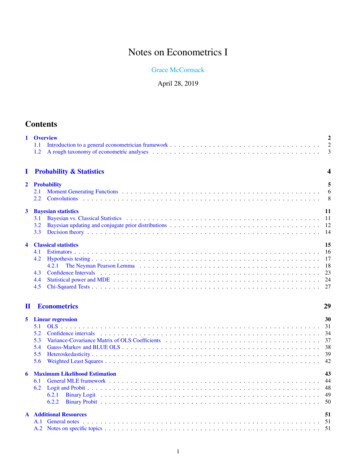
3.2Bayesian updating and conjugate prior distributions13Consider if we have a coin with unknown probability θ [0, 1] of flipping heads. We want to know the probability that the coinunfairly favors heads (i.e. θ /f rac12). We have some prior belief about the likelihood of different θ values being the true θ, butwe want to use data to update this belief. To do so, we will be flipping coins and updating our prior to generate a posterior distribution.Example 1: flat priorSet upPriorExperimentResult(θ)θ 2θf (θ x)f (θ x) R 1 ff(x θ)f R θdθ(x θ)f (θ)dθ0R1P r(unfair coin) P r(unfair coin) 1/2 2θdθ 43Example 2: H-favored priorSet upPriorExperimentResult(θ)2θ 22 R 2θf (θ x)f (θ x) R 1 ff(x θ)f2 dθ 3θ(x θ)f (θ)dθ0R1P r(unfair coin) P r(unfair coin) 1/2 23θ2 dθ 87Example 3: Flat prior, more dataSet upPriorExperimentResult2(θ)f (θ x)f (θ x) R 1 ff(x θ)f R θθ2 dθ 3θ2(x θ)f(θ)dθ0R1P r(unfair coin) P r(unfair coin) 1/2 23θ2 dθ 34f (θ) 11 coin flipHf (θ) 2θ1 coin flipHf (θ) 2θ1 coin flipHH
3.33.3Decision theory14Decision theoryDecision theory studies how agents make choices under uncertainty and has two main branches: a normative philosophical side anda more formal mathematical side. We shall be giving the briefest introduction to the latter. You might notice that it is closely relatedto what you are already learning in your first semester of microeconomics.The main idea: We consider an individual who may take action α1 .αj (For example α1 invest, α2 not invest) Each of these actions is associated with some distribution of utility values associated with possible outcomes (For example,f1 (u) might be the distribution of possible returns on investment) Individuals are expected utility maximizers - that is, when faced with multiple options, they will choose the option that willgive them the highest value in expectation given the information that htey have.R– The chosen action α argmaxj { ufj (u)} In our example, even though an individual may “win” or “lose” on an investment, they will still invest if the investment willpay off in expectation.The value of information New information can change your behavior; for example, if the individual from the previous example has a machine thatperfectly predicts if the investment pays off, they will only invest in “winners” and never invest in “losers.” Consider information I that changes the distribution of possible utilities fjI so that we have more certainty over what shalloccur– Under perfect information, fjI will be degenerate, giving you a perfect prediction of what will happen– Under imperfect information, fjI will not give you perfect omniscience, but will give you a more accurate picture of thefuture than no information If information changes your behavior, it also changes your expected utility; we can calculate the expected utility that individualsget under different levels of information– EV P I – the expected value that an individual will get under perfect information– EV II – the expected value that an individual will get under imperfect information– EV N I – the expected value that an individual will get under no information (this is the baseline in most situations) We can use these expected values to derive the incremental value of different pieces of information– V P I EV P I EV N I , the additional value that individuals get from having perfect infromation relative to no information. You can think of this as the willingness to pay for that information– V II EV II EV N I , the additional value that individuals get from having imperfect infromation relative to noinformation.– Typically, V P I V II
154Classical statisticsWhile Bayesian Statistics makes a lot of sense, it does presentsome difficulties as an empirical framework. For one, it requiresus to take a stance on what prior to use. While some sitationsmight elicit a natural prior, researchers will often end up arguingover the appropriate prior. A researcher hungry for citationsmight be tempted to use whatever prior that will generate a moredramatic finding. Further, because Bayesian statistics typicallyresults in posterior distributions of a parameter θ, not necessarily asingle “point estimate,” it is less clear as a way to present material(though this limiation can be overcome for some BayesianEstimators).Classical Statistics (sometimes called Frequentist Statistics)is the dominant type of statistical framework for the sciencesand social sciences. The main distinction between Bayesian andClassical is that we no longer have to choose a prior. The onlything that matters for estimation and inference is the data weobserve.There are a couple inter-related concepts with which wewill have to become comfortable as we dive into ClassicCalStatistics:1. Estimators - our “best guess” θ̂ of a parameter θ2. Hypothesis test - a process of deciding whether or not toreject hypotheses at certain “confidence levels” based on thedata we observe3. Power and MDE - given a desired hypothesis test, a way toassess how we want to design our experiment to make surewe will be able to draw meaningful conclusions from ourdata4.
policy design. In this vein, I wish us to think of econometrics as a means of using data to understand something about the true nature of the world. The organizing framework for these notes can be seen below. I will be returning to this framework throughout the notes. . PhD course and that there are several