WIXLIB

IntroductionRepetition of statistical terminologySimple linear regression modelEstimateNotation for estimates and parametersParameters are usually denoted by Greek letters: α,β,θ,. . .The corresponding estimates or estimators are denoted by a hat:α̂, β̂, θ̂, . . . Latin letters (a estimates α etc.) are also used by someauthors.Introductory EconometricsUniversity of Vienna and Institute for Advanced Studies Vienna

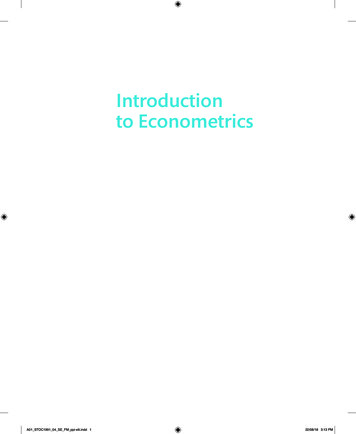
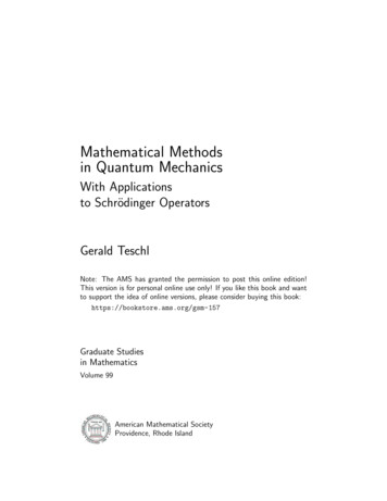
IntroductionRepetition of statistical terminologySimple linear regression modelEstimate708090100C110120130Examples of estimators100120140YDConsumption C depending on income YD can be represented as a consumption function (line) and as data pointsin a scatter diagram: the intercept α̂ estimates the autonomous consumption, the slope β̂ estimates the marginalpropensity to consume of the households.Introductory EconometricsUniversity of Vienna and Institute for Advanced Studies Vienna

IntroductionRepetition of statistical terminologySimple linear regression modelTestDefinition of the hypothesis testA test is a statistical decision rule. The aim is a decision whetherthe data suggest that a specified hypothesis is incorrect (‘toreject’) or correct (‘not to reject’, ‘to accept’, ‘fail to reject’).It is customary first to calculate a test statistic from the data, areal number that is a function of the data. If this statistic is in therejection region (critical region), the test is said to reject.Introductory EconometricsUniversity of Vienna and Institute for Advanced Studies Vienna

IntroductionRepetition of statistical terminologySimple linear regression modelTestTests: common mistakes A test is not a test statistic. The test statistic is a realnumber, whereas the test itself can only indicate rejection oracceptance (‘non-rejection’), a decision that may be coded by0/1. A test cannot be 1.5. A test is not a null hypothesis. A test cannot be rejected.The tested hypothesis can be rejected. The test rejects.Introductory EconometricsUniversity of Vienna and Institute for Advanced Studies Vienna

IntroductionRepetition of statistical terminologySimple linear regression modelTestDo economic theories deserve a presumption of innocence?The null hypothesis (or short null) is a (typically sharp) statementon a parameter. Example: β 1. These statements oftencorrespond to an economic theory.The alternative hypothesis (or short alternative) is often thenegation of the null within the framework of a general hypothesis(maintained hypothesis). Example: β (0, 1) (1, ). Thisstatement often corresponds to the invalidity of an economictheory.Notation: H0 for the null hypothesis and e.g. HA for thealternative. H0 HA is the general or maintained hypothesis.Example: the maintained hypothesis β 0 is not tested butassumed (‘window on the world’).Introductory EconometricsUniversity of Vienna and Institute for Advanced Studies Vienna

IntroductionRepetition of statistical terminologySimple linear regression modelTestHypotheses: common mistakes A hypothesis cannot be a statement on an estimate.“H0 : β̂ 0” is meaningless, as β̂ can be determined exactlyfrom data. Alternatives cannot be rejected. The classical hypothesestest is asymmetrical. Only H0 can be rejected or ‘accepted’.(Bayes tests are non-classical and follow different rules) Hypotheses do not have probabilities. H0 is never correctwith a probability of 90% after testing. (Bayes tests allotprobabilities to hypotheses)Introductory EconometricsUniversity of Vienna and Institute for Advanced Studies Vienna

IntroductionRepetition of statistical terminologySimple linear regression modelTestErrors of type I and of type IIThe parameters are unobserved and can only be determinedapproximately from the sample. For this reason, decisions are oftenincorrect: If the test rejects, although the null hypothesis is correct, thisis a type I error; If the test accepts the null, although it is incorrect, this is atype II error.A basic construction principle of classical hypothesis tests is toprescribe a bound on the probability of type I errors (e.g. by 1%,5%) and, given this bound, to minimize the probability of a type IIerror.Introductory EconometricsUniversity of Vienna and Institute for Advanced Studies Vienna

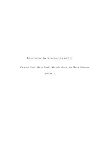
IntroductionRepetition of statistical terminologySimple linear regression modelTest0.00.10.20.30.4Two tests on a 5% level 4 2024Density of a test statistic under H0 . 2 tests use the same test statistic.The one with red rejection region is viewed as a worse test than the onewith green rejection region, as it implies more type II errors.Introductory EconometricsUniversity of Vienna and Institute for Advanced Studies Vienna

IntroductionRepetition of statistical terminologySimple linear regression modelTestMore vocabulary on testsThe often pre-specified probability of a type I error is called thesize of the test or the significance level. For simple nullhypotheses, it will be approximately constant under H0 , otherwiseit is an upper bound.The probability not to make a type II error is called the power ofthe test. It is defined on the alternative, and it depends on the‘distance’ from H0 . Close to H0 , power will be low (close to size);at locations far from H0 , it approaches 1.If the test attains a power of 1 on the entire alternative, as thesample size grows toward , the test will be called consistent.Introductory EconometricsUniversity of Vienna and Institute for Advanced Studies Vienna

IntroductionRepetition of statistical terminologySimple linear regression modelTestBest testsA concept analogous to efficient estimators, a test that attainsmaximal power at given size, exists for some simple problems only.For most test problems, however, the likelihood-ratio test (LR test,the test statistic is a ratio of the maxima of the likelihood underH0 and HA ) has good power properties.Often, the Wald test and the LM test (Lagrange multiplier)represent ‘cheaper’ approximations to LR and still they haveidentical properties for large n .Attention: LR, LM and Wald test are construction principles fortests, not specific tests. It does not make sense to say that ‘theWald test rejects’, unless it is also indicated what is being tested.Introductory EconometricsUniversity of Vienna and Institute for Advanced Studies Vienna

IntroductionRepetition of statistical terminologySimple linear regression modelTestCan a presumption of innocence apply to the invalidity of atheory?Economic statements need not correspond to the null of ahypothesis test. Sometimes, the null hypothesis is the invalidity ofa theory. For example, theory may tell that the export ratiodepends on the exchange rate.Even then, the null of the test corresponds to the more restrictivestatement. The economic statement becomes the alternative. Theinvalidity of the economic theory can be rejected. For example, H0says that the coefficient of the export ratio that depends on theexchange rate is 0, and this is rejected.Introductory EconometricsUniversity of Vienna and Institute for Advanced Studies Vienna

IntroductionRepetition of statistical terminologySimple linear regression modelp–valuesHow are significance points found?Tests are usually defined by a test statistic and by critical values.Critical values (significance points) are usually quantiles of thedistribution of the test statistic under H0 .Determination of critical values:1. Tables: Quantiles of important distributions have beentabulated by simulation or by analytical calculation.2. Calculation: Computer inverts the distribution function.3. p–values: Computer calculates marginal significance levels.4. Bootstrap: Computer simulates distribution function under H0and takes characteristics of the sample into account.Introductory EconometricsUniversity of Vienna and Institute for Advanced Studies Vienna

IntroductionRepetition of statistical terminologySimple linear regression modelp–valuesDefinition of the p–valueCorrect definitions: The p–value is the significance level, at which the testbecomes indifferent between rejection and acceptance for thesample at hand (the calculated value of the test statistic); The p–value is the probability of generating values for the teststatistic that are, under the null hypothesis, even moreunusual (less typical, often ‘larger’) than the one calculatedfrom the sample.Incorrect definition: The p–value is the probability of the null hypothesis for thissample.Introductory EconometricsUniversity of Vienna and Institute for Advanced Studies Vienna

IntroductionRepetition of statistical terminologySimple linear regression modelp–values0.00.10.20.30.4Test based on quantiles 4 202410% to 90% quantiles of the normal distribution. The observed value of2.2 for the test statistic that is, under H0 , normally distributed issignificant at 10% for the one-sided test.Introductory EconometricsUniversity of Vienna and Institute for Advanced Studies Vienna

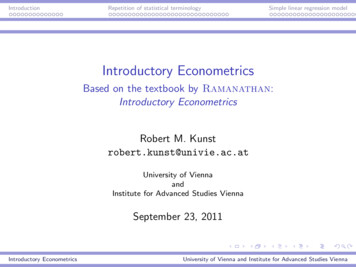
IntroductionRepetition of statistical terminologySimple linear regression modelp–values0.00.10.20.30.4Test based on p–values 4 2024The area under the density curve to the right of the observed value of 2.2is 0.014, which yields the p–value. The one-sided test rejects on thelevels of 10%, 5%, but not 1%.Introductory EconometricsUniversity of Vienna and Institute for Advanced Studies Vienna

IntroductionRepetition of statistical terminologySimple linear regression modelExpectation and varianceDefinition of expectationThe expectation of a random variable X with density f (x) isdefined byZ EX xf (x)dx. For discrete random variables with probabilities P(X xj ), thecorresponding definition isE(X ) nXxj P(X xj ).j 1Introductory EconometricsUniversity of Vienna and Institute for Advanced Studies Vienna

IntroductionRepetition of statistical terminologySimple linear regression modelExpectation and varianceLinearity of expectationFor two (even dependent) random variables X and Y and arbitraryα R,E(X αY ) EX αEY ,holds, and the expectation of a constant ‘random variable’ a is a.Beware, however, that in general E(XY ) 6 E(X )E(Y ), andEg (X ) 6 g (EX ) for a general function g (.), particularlyE(1/X ) 6 1/EX .Introductory EconometricsUniversity of Vienna and Institute for Advanced Studies Vienna

IntroductionRepetition of statistical terminologySimple linear regression modelExpectation and varianceEstimation of the expectationThe most usual estimator for the expectation of a random variableis the sample meannXX̄ Xt /n .t 1Pair of concepts: Expectation EX : population mean, parameter, unobserved. Mean X̄ : sample mean, statistic, observed.Introductory EconometricsUniversity of Vienna and Institute for Advanced Studies Vienna

IntroductionRepetition of statistical terminologySimple linear regression modelExpectation and varianceDefinition of the varianceThe variance of a random variable X with density f (x) is defined byvarX E(X EX )2 EX 2 (EX )2 .It measures the dispersion of a random variable around itsexpectation (centered 2. Moment). A customary notation isσX2 varX .The square root of the variance is called the standard deviation(preferred for observed X ) or standard error (preferred forstatistics) and is often denoted by σX .Introductory EconometricsUniversity of Vienna and Institute for Advanced Studies Vienna

IntroductionRepetition of statistical terminologySimple linear regression modelExpectation and varianceProperties of the variance1. varX 0;2. X α R varX 0;3. var(X Y ) varX varY cov(X , Y ) withcov(X , Y ) E{(X EX )(Y EY )};4. α R var(αX ) α2 varX .The variance operator is not linear, varX can also be .Introductory EconometricsUniversity of Vienna and Institute for Advanced Studies Vienna

IntroductionRepetition of statistical terminologySimple linear regression modelExpectation and varianceEstimation of the varianceThe most customary estimator for the variance of a randomvariable is the empirical variancevar(Xc ) nnt 1t 11 X1 X 2n(Xt X̄ )2 Xt X̄ 2 .n 1n 1n 1Pair of concepts: Variance varX : population variance, parameter, unobserved. Sample variance varXc : statistic, observed.Introductory EconometricsUniversity of Vienna and Institute for Advanced Studies Vienna

IntroductionRepetition of statistical terminologySimple linear regression modelProperties of estimatorsBias of estimatorsSuppose θ̂ is an estimator for the parameter θ. The valueEθ̂ θis called the bias of the estimator. If the bias is 0, i.e.Eθ̂ θ,then the estimator is called unbiased. This is certainly a desirableproperty for estimators: the distribution of the estimates iscentered around the true value.Introductory EconometricsUniversity of Vienna and Institute for Advanced Studies Vienna

IntroductionRepetition of statistical terminologySimple linear regression modelProperties of estimatorsConsistency of estimatorsAssume that the sample size diverges toward . Denote theestimate for the sample size n by θ̂n . If, in any reasonabledefinition of convergenceθ̂n θ, n ,then the estimator is called consistent. This is another desirableproperty of estimators: the distribution of the estimates shrinkstoward the true value, as the sample size grows.Introductory EconometricsUniversity of Vienna and Institute for Advanced Studies Vienna

IntroductionRepetition of statistical terminologySimple linear regression modelProperties of estimators0.00.20.40.60.81.0Consistency is more important than unbiasedness 4 2024Consistent estimator with bias for the true value of 0. Small sample red,intermediate green, largest blue.Introductory EconometricsUniversity of Vienna and Institute for Advanced Studies Vienna

IntroductionRepetition of statistical terminologySimple linear regression modelProperties of estimatorsConsistency and unbiasedness do not imply each otherExample: Let Xt be independently drawn from N(a,1). Someonebelieves a priori b to be a plausible value for the expectation.â1 X̄ b/n is consistent, usually biased, and a reasonableestimator.Example: Same assumptions, â2 (X1 Xn )/2 is unbiased, butinconsistent and an implausible estimator.These examples are constructed but typical: inconsistent estimatorsshould be discarded, biased estimators can be useful or inevitable.Introductory EconometricsUniversity of Vienna and Institute for Advanced Studies Vienna

IntroductionRepetition of statistical terminologySimple linear regression modelProperties of estimatorsEfficiency of estimatorsAn unbiased estimator θ̂ is called more efficient than anotherunbiased estimator θ̃, ifvarθ̂ varθ̃.If θ̂ has minimal variance among all unbiased estimators, it iscalled efficient.Remark: Excluding biased estimators is awkward, but we will workwith this definition for the time being.Introductory EconometricsUniversity of Vienna and Institute for Advanced Studies Vienna

IntroductionRepetition of statistical terminologySimple linear regression modelSimple linear regressionThe model explains (describes) a variable Y by a variable X , withn observations available for each of the two:yt α βxt ut ,t 1, . . . , n,where α and β are unknown parameters (coefficients). Theregression is called simple, as only one variable is used to explain Y ; linear, as the dependence of Y on X is modelled by a linear(affine) function.Introductory EconometricsUniversity of Vienna and Institute for Advanced Studies Vienna

IntroductionRepetition of statistical terminologySimple linear regression modelTerminologyIn words, Y is said to be regressed on X .Y is called the dependent variable of the regression, also theregressand, the explained variable, the response;X is called the explanatory variable of the regression, also theregressor, the design variable, the covariate.Usage of the wording ‘independent variable’ for X is stronglydiscouraged. Only in true experiments will X be set independently.In the important multiple regression model, typically all regressorsare mutually dependent.Introductory EconometricsUniversity of Vienna and Institute for Advanced Studies Vienna

IntroductionRepetition of statistical terminologySimple linear regression modelα and βα is the intercept of the regression or the regression constant. Itrepresents the value for x 0 on the theoretical regression liney α βx, i.e. the location where the regression line intersectsthe y –axis. Example: in the consumption function, α isautonomous consumption.β is the regression coefficient of X and indicates the marginalreaction of Y on changes in X an. It is the slope of the theoreticalregression line. Example: in the consumption function, β is themarginal propensity to consume.Introductory EconometricsUniversity of Vienna and Institute for Advanced Studies Vienna

IntroductionRepetition of statistical terminologySimple linear regression modelWhat is u?In the descriptive regression model, u is simply the unexplainedremainder.In the statistical regression model, the true ut is an unobservedrandom variable, the error or disturbance term of the regression.The word ‘residuals’ describes the observed(!) errors that evolveafter estimating coefficients. Some authors, however, call theunobserved errors ut ‘true residuals’.Introductory EconometricsUniversity of Vienna and Institute for Advanced Studies Vienna

IntroductionRepetition of statistical terminologySimple linear regression modelIs simple regression an important model?The simple linear regression model offers hardly anything newrelative to correlation analysis for two variables, and it is ratheruninteresting.It is a didactic tool that permits to introduce new concepts thatcontinue to exist in the multiple regression model. This multiplemodel is the most important model of empirical economics.Introductory EconometricsUniversity of Vienna and Institute for Advanced Studies Vienna

IntroductionRepetition of statistical terminologySimple linear regression modelThe descriptive linear regression problemDescriptive regressionThe descriptive problem does not make an

Introductory Econometrics Based on the textbook by Ramanathan: Introductory Econometrics Robert M. Kunst robert.kunst@univie.ac.at University of Vienna and Institute for Advanced Studies Vienna September 23, 2011 . Econometrics Selected