Transcription
Getting Started With Microcal Origin 6For Windows NTAn introduction to theMicrocal Origin scientificcharting package.AUTHORInformation Systems ServicesUniversity of LeedsDATEDecember 1999EDITION1TUT7775p
ContentsIntroductionAim of this DocumentWhat Is Origin?111Task 1 Running Microcal Origin2Task 2 Creating a Simple Graph4Task 3 Editing Graphic Elements8Task 4 Obtaining Printed Output12Task 5 Importing Data Files13Task 6 Multiple Graphs on the Same Page14Task 7 Curve Fitting : Pre-Defined15Task 8 Curve Fitting : User-Defined18Task 9 Creating a 3D Graph20Task 10 Creating a Surface Plot23Task 11 Quitting Origin25Further InformationOn-line HelpDocumentation262626Appendix 1 Types of Graph Available2D Graphs3D Graphs272728Appendix 2 Origin Examples30Format ConventionsIn this document the following format conventions are used:Commands that you must type in are shownin bold Courier font.Input which must be replaced by your detailsis given in italicsMenu items are given in a Bold, Arial font.Keys that you press are enclosed in anglebrackets.WIN31LOGIN server/usernameWindows Applications Enter FeedbackIf you notice any mistakes in this document please contact the Information Officer.Email should be sent to the address a.clough@leeds.ac.ukCopyrightThis document is copyright University of Leeds. Permission to use materialin this document should be obtained from the Information Officer (emailshould be sent to the address info-officer@leeds.ac.uk)Print RecordThis document was printed on 14-Mar-00.
IntroductionAim of this DocumentThis document describes the Microcal Origin 3D module program. Thedocument is intended for new users. It describes the basic features availablein Origin and gives advice on printing and including data from externalsources. It also includes a simple exercise in the use of Origin.What Is Origin?Origin is a technical graphics and data analysis software. It is fast, powerful,easy to use and ideal for anyone who needs advanced graph plotting, datahandling and analysis. With its drawing tools, Origin provides flexibility increating complex graph and publication quality output. Origin provides agraphing environment where you can enter your data, or import data filesfrom other applications, to create professional looking graphs, and outputthem on a variety of devices.Origin 6 is available on the Novell network under Windows NT. Users withstandalone PCs can purchase the software from the ISS. The ISS can alsosell networked versions of the software for installation on departmentallymanaged PC networks.1
Task 1 Running Microcal OriginObjectiveTo run Microcal Origin.Instructions You will need to run Windows NT. If you are using a PC on a computernetwork you will first need to login to the network.CommentsYou will need to have access to a PC which runs Windows NT in order tocarry out this activity.Activity 1.1Open Windows NT and click on Start Programs Graphics Origin 6(see Figure 1).(Your desktop may look slightly different if you are not logged on to theInformation Systems Services network. If this is the case, you may need toask your departmental Computer Officer if and where Origin 6 has beeninstalled.)NoteOrigin 6 can also be run from ZENworks (see Figure 2). For information onhow to get ZENworks - Open a web browser such as Netscape and go to thefollowing URL: http://www.leeds.ac.uk/iss/NT/zenworks.htmlFigure 1. Finding Origin 6 on theWindows NT desktopFigure 2. Finding Origin 6 inZENworks2
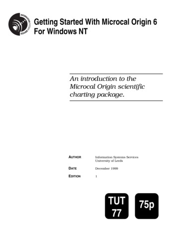
The screen shown in Figure 3 is displayed.Figure 3. The Origin screenActivity 1.2Ensure that all menu options will be available for the session by checkingFull Menus from the Format, Menu menu, as shown in Figure 4. When it isselected, it has a bullet against it, as shown.Figure 4. Menu selection3
Task 2 Creating a Simple GraphObjectiveCreating a simple graph.Instructions Enter data into the worksheet and create a graph.CommentsType in the data as shown.Activity 2.1The default number of columns is two. In this example we require threecolumns of data. To add another column to the worksheet, click on theColumn menu and choose the Add New Columns. option or click on the iconfrom the toolbar. Click OK to add the default number of columns, 1. Anextra column named C(Y) isadded.Activity 2.2Enter some data into theworksheet as shown in Figure 5.Change the name of column C byclicking on the column C(Y)heading. Select the Columnmenu and then the Set as Y Erroroption. Column C will now showthe heading C(yEr ), as shownin Figure 5.Figure 5. Entering dataActivity 2.3 Un-highlight column C.Click on the Plot menuand choose theLine Symbol graph. Youare then given theopportunity to select thevalues you want todisplay, as shown inFigure 6, the SelectColumns for Plottingdialog box. HighlightA(X) in the left handcolumn and then click onbutton. Thisthetells Origin to put datafrom column A along theX Axis.Next, highlight B(Y) inFigure 6. Selecting the columns to plotbutton. This tells Originthe left hand column and then click on theto put data from column B along the Y Axis. Click on the OK button whenyou have finished.4
Activity 2.4A new plot window appearsshowing Column B plottedagainst Column A onto adefault set of axes. Alegend automaticallyappears at the upper rightcorner of the window,showing the data set name,and plot type as shown inFigure 7.The data set name in thisexample is B as that is thecurrent column heading.This can be changed tosomething more descriptivein two ways:Figure 7. A Line Symbol plot change the legend entry in the graph window, or change the column heading in the worksheet.Activity 2.5To change the legend entry in the graph window, double-click on the item inthe legend (in this case the letter B). The following dialog box appears:The characters in themiddle box indicatewhat will be displayedin the legend. In thisexample, L(1) meansthat the linestyle andcolour of line number1 will be displayedand %(1) means thatthe column headingfor the first plotteddataset will bedisplayed. To changethe text, delete %(1)and enter therequired text asshown in Figure 9.Figure 8. Entering legend textThe format of thelegend text is shownin the bottom section of the Text Control dialog box (also shown in Figure 9).5
Press OK . The new textshould now appear in thelegend.Figure 9. The revised legend textActivity 2.6To change the legend by renaming the required column, double-click on therequired column in the worksheet. The following dialog box appears:Enter the new nameinto the Column Labeland press OK .Choose whether todisplay the ColumnLabel in the Datawindow. The legendin the graph will notbe updatedautomatically – toupdate it, click on thegraph window andthen click on Graph,New Legend. Thegraph legend will beupdated.Figure 10. Renaming columnsActivity 2.7Plotting error bars is very simple. You could do it when you create theLine Symbol plot by selecting Column C and entering it using thebutton, as shown in Figure 6. Alternatively, as in this example, you may adderror bars once you have created the Line Symbol plot.Error bars can be added to plots in two different ways: to add error bars thatyou wish to be computed as a percentage or a standard deviation of the data- select the Add Error Bars. option from the Graph menu.6
For this example, we will add error bars from a dataset – double click on thelayer icon in the top left hand corner of the plot window. The Layer dialogbox (Figure 11) appears. Select the dataset that you want to use from theto add it to the layer.Available Data – in this case data1 c – and pressAs the column has already been defined as error bars, that is what will beplotted. Press OK .Figure 11. The Layer dialog boxThe plot is now redrawn with error bars, as shown in Figure 12 below:Figure 12. A Line Symbol plot with error barsTo zoom in and out of a graph, use the zoom icons on the main toolbar.Choose View, Whole Page to return the graph to its original size and position.7
Task 3 Editing Graphic ElementsObjectiveTo edit the graphic elements of a plot.Instructions You will edit the graph style and colours and use the Tools toolbar to add atext label.CommentsExperiment by editing the other graphic elements as well.Activity 3.1Editing graphs in Origin is straightforward. Each graph is composed of avariety of graphic elements. To change any element, you must position themouse on that element and double-click the left hand mouse button. Figure13 shows most of the graphic elements that can be edited by double-clicking.Figure 13. Editing graphic elementsActivity 3.2Double click on one of the datapoints on the graph: the dialog box thatappears (Figure 14) enables you to change the graph type, the colours, linestyles, shapes of data points etc. Click on the Line tab and change the typeof line to spline andmake it a dotted violetline with no gapbetween the line andthe data points. Press OK . This willproduce a curve whichpasses through thedata points.Figure 14. The Plot Details dialog box8
Most elements on the graph are grouped with other similar elements - forexample if you double click on one of the data points and change its colour,all the other data points for that dataset will also change. If you want tooverride this grouping, hold down the CTRL key when you double clickover the point and any changes that you then make will affect only theselected point.Activity 3.3Hold down the CTRL key and double click over a data point, change thecolour to red. The selected point should be the only one that changes. Thisis a good way to highlight individual points.Activity 3.4Alternatively, elements can also have their attributes selected automaticallyusing column values. Add a fourth column to the worksheet as in activity2.1 and enter the following values into it: 4,2,4,2,4. Highlight the first 3columns and select Plot Line and Symbol – this is a quicker way toproduce a plot than activity 2.3. Double click on one of the data points onthe new graph. In the Plot Details dialog box choose the Symbol tab. Fromthe Symbol Color list choose Indexing, Col(D). Check the Show Constructionbox and from the Shape drop down menu choose Col(D). Press OK . Theresulting plot should show some points as blue triangles and others as redcircles.Activity 3.5To add text to a graph, for example atitle, it is necessary to use the toolstoolbar. If the Tools toolbar is notavailable it may have been switchedFigure 15. The Tools toolbaroff. To open this toolbar, click on theView, Toolbars menu option. From the toolbars dialog box select Tools. Itshould now be displayed.The first six tools from the left are used mainly for working with data in plotwindows. The next six are used to add labels to a graph or to a worksheet. Adetailed description of these tools is available in the Origin User’s Manual.To add a title tothe first plot, forexample, click onthe Text tool andposition the cursoras desired in theplot window.Click again andthe Text Controldialog box willappear, as shownin Figure 16. Typethe desired textwhere it highlights‘enter texthere’ and clickon the OK button. The titlewill now appear onthe plot.Figure 16. Text Control dialog box9
Special characters such as and Greek characters can be inserted by typing****, where **** is the ASCII code for the required symbol. Note - theASCII code must be typed on the number pad of the keyboard while holdingdown the Alt key. e.g. 0174 gives the symbol Activity 3.6Items in columns can also be used for labels:Highlight Column A, select Column Set as Label. Enter labels into ColumnA, overwriting the numbers e.g. sample 1, sample 2, sample 3, sample4, sample 5.Note - Column A no longer represents the x data; if there is no x columnselected then Origin will use the row numbers by default.In the Graph window, double click on one of the numbers under the x axis.In the dialog box, choose the Tick Labels tab and select Text from dataset asthe tick label Type and then Data1 A as the Dataset. Click OK and thegraph should now look like:Figure 17. The graph with the x-axis labelledTo add more data to a graph, you can simply type in more data into columnsthat are already plotted – the graph should automatically redraw.Activity 3.7To add complete new datasets to a graph, add a new column to theworksheet as before, add the new data into Column E. Double click on thelayer icon in the top left hand corner of the graph window. The box shown inFigure 18 appears.10
Figure 18. Adding another datasetbutton to add the dataset to the LayerSelect data1 e and press theContents box. Press OK . The new data should now appear on the graphalongside the first dataset, as in Figure 19, and can be edited in the sameway. Datasets can also be deleted from graphs by using thebutton.Figure 19. The graph showing the new datasetTo update the legend, select Graph New Legend, or press the New Legendicon on the main toolbar, and then alter the legend text as shown previously.11
Task 4 Obtaining Printed OutputObjectiveTo obtain a printed copy of your graph.Instructions You will use the Print Setup dialog box to attach to a printer.CommentsMake sure that you attach to the correct printer.Activity 4.1Before you print your graph you must make sure that you are connected tothe correct printer. (You will normally find that each printer is labelled withits name.)From within Origin, select File Print. Click on the drop-down menu byName and select a printer.Activity 4.2You can set your paper size, orientation and other settings using theDocument Properties dialog box which can be accessed by selecting theProperties button. Figure 20 shows the Print dialog box.Figure 20. Print Setup dialog boxActivity 4.3Create and edit your graphs as previously described. Select File Print toprint a single graph.Note You may want to print several graphs on the same page. To do thisselect File New Layout. A new window should appear with a blank pageon it. Use the Layout Add Graph and Add Worksheet options to positiongraphs and tables on the blank page for printing. Size the graphs andworksheets on the layout page and align using the Object Edit tools whichcan be accessed by selecting View Toolbars and selecting Object Edit. TheObject Edit palette shown in Figure 21 provides tools which allow for easyarrangement of objects. The action of each button is explained in the OriginUser’s Manual.Figure 21. TheObject Edit Menu12
Task 5 Importing Data FilesObjectivesTo import data from another format.Instructions You will import an ASCII file.CommentsYou need to be using a networked PC to use example data files.In Origin, it is possible to import data from other formats. The importformats include ASCII, Lotus, Excel, dBase, Symphony, sigmaplot, soundwave and Dif. The export formats include ASCII files, WMF, EPS and BMP.For this example we will import an ASCII file.Activity 5.1Open a new worksheet by selecting File New Worksheet. Click on theFile menu and then choose the Import Single ASCII option. The File Opendialog box should appear listing files with a .dat extension. Figure 22shows the File Open dialog box.Figure 22. File Open dialog boxIf no files are listed make sure you are in the correct directory:L:\win32apps\Origin41\SamplesClick on the test3.dat file name and then click Open. The ASCII file test3is now open in Origin. You might also use cut/copy/paste or DDE (DynamicData Exchange) with Origin. DDE is a Windows feature that enablescommunication between applications that run under windows. DDE allows agraph in Origin to be dynamically linked to data in another windowsapplication that supports DDE, such as Excel. When you alter the data inExcel, the graph in Origin is automatically updated to reflect the changes.You can also use DDE to paste Origin graphs into a word processing packagesuch as Word for Windows. The Paste Link command in the Edit menu isused to create DDE links in Origin.13
Task 6ObjectivesMultiple Graphs on the Same PageTo plot two different graphs on the same page.Instructions You will import an additional data file into the document.CommentsYou need to be using a networked PC to use example data files.Activity 6.1You should already have test3.dat imported into Origin from the previousexample; if not, do it now.Activity 6.2Highlight the Column Cp by clicking on the Cp(Y) heading. Open the Plotmenu and choose the Line option. The first data set and graph has now beenproduced.Activity 6.3Now select the New, Worksheet option from the File menu and import theASCII data file TEST2.DAT as previously. Highlight Column B by clicking onthe B(Y) heading and choose the Line option from the Plot menu. Graph 2will now open containing a second graph.Activity 6.4Make sure that Graph 1 and Graph 2 are the only windows open. Click on theGraph 1 window to make it active and choose the Merge All Graph Windowsoption from the Edit menu. A dialog plot will appear asking if you want tokeep the old plots – click on YES. You then get the layering and spacingoptions, choose the default settings for now by clicking OK . The twographs will appear Graph 2 below Graph 1.Click on the Edit menu and choose the Add & Arrange Layers. option. Click OK and then alter the vertical gap from 5 to 10. Click OK . This will adda little more vertical space between the plots. The following plot should nowappear:Figure 23. Two graphs on the same page14
Task 7 Curve Fitting: Pre-DefinedObjectiveTo introduce the concepts of curve fitting.Instructions You will use as an example a pre-defined function.CommentYou need to be using a networked PC to use example data files.When you are in a Graph window, Origin’s linear and polynomial fit menucommands are located in the Analysis menu. Parameter initialization andfitting is carried out automatically when fitting from the menu. A fit curve isdisplayed in the graph window while the fitting parameters and statisticalresults are recorded in the Script window.The Analysis menu contains the most frequently used models which include: Linear Regression Polynomial Regression Exponential Decay (first order, Second order and Third order) Exponential Growth Gaussian (single & Multiple) Lorentzian (single & Multiple) Sigmoidal Multiple Peaks Non-linear curve fit (one of the above or User defined one)Users can add their own fitting function or have more control over fittingparameters by using the Nonlinear Curve Fit option from the Analysis menu.Activity 7.1Consider a curve fitting session using one of the pre-defined functions. Totry this example you should open the file fitexmp1.opj which is availableunder L:\win32apps\Origin41\Samples. Figure 24 shows the plot whichwill be used for the example.Figure 24. Scatter graph15
From the Analysis menu choose the Fit Exponential Decay - First Orderoption. Origin will do the necessary initialization and fit the data. The resultof this operation is shown in Figure 25:Figure 25. "First order – exponential decay" curve fittingA Script Window also appears, giving details of the fitting parameters.Activity 7.2In the above case the X offset is assumed zero by the auto initialization. Toallow an X offset you should choose the Non-Linear Curve Fit option from theAnalysis menu. A new set of menus is displayed and the following dialog boxappears: Click Select Function andchoose ExpDecay1 fromthe functions list. Click Start Fitting,followed by Yes. Make sure the Vary?check box for x0 ischecked Click 1 iter. button onthe menu bar and thenclick Done on the menubarFigure 26. Fitting Session Dialog BoxThis will update the plot and the contents of the Script Window with the newfitting parameters.Figure 26 shows the basic NLCF Mode. The advanced NLCF mode can beaccessed by clicking on the More button from the basic mode (see Figure 27).16
While both modes enable you to fit your data, they differ substantially in theoptions they provide as well as in the degree of complexity they entail.The basic mode is simpler and is used for selecting a function, selectingdatasets for fitting, performing an iterative fitting procedure and displayingthe results on the graph.The advanced mode includes the above and allows the user to define a scriptto initialize parameters, impose linear constraints, define your own fittingfunction, specify a weighting method and termination criteria, displayconfidence and prediction bands, residue plot, parameter worksheet, and thevariance-covariance matrix. It also allows the user to fit multiple datasetswith a choice of shared parameters and change parameter names.Figure 27. Advanced NLCF Mode17
Task 8 Curve Fitting: User-DefinedObjectivesCurve fitting using a User-defined function.Instructions You will use an example of a User-defined function.CommentsYou need to be using a networked PC to use example data files.Activity 8.1Consider a curve fitting session using a user-defined function. To try thisexample you should open the file fitexmp2.opj which is available underL:\win32apps\Origin41\Samples.To enter a new fitting function, from the Analysis menu choose the Non-linearcurve Fit option. The following dialog box will be displayed:Figure 28. Select a new functionFigure 29. Define a new fit functionClick on the New button. From the Edit Function Menu enter 3 in theNumber of Param. box. Next enter the following into the Definition box at thebottom:P1*exp(-x P2/P3)and click the Save and then the Accept button.Activity 8.2To start the fitting session from the menu in Fig. 28, click on the Start Fittingbutton. You will be prompted for a choice of fitting the curve for the activedata set or any other. Choose the active dataset. The fitting session menuappears and you need to set the starting values for P1, P2, P3 in the boxesadjacent to the parameters e.g. try P1 7, P2 2, P3 2.If you want to fix the value of any of the parameters you must click on thebox next to the value box that says Vary? as shown in Figure 30. If theVary? boxes are checked it allows the parameters’ values to change duringthe iterations.Click in the 1 Iter. or 10 Iter. box to do the curve fit. Repeat the iterationsuntil you get a satisfactory fit. Once you are happy with the curve, click theDone button to terminate the fitting session.18
Figure 30. Fitting session menuFigure 31 shows the result of fittingthe function to the plot.NoteThe option More. during the Fittingsession provides the user with moresophisticated options to control thefitting parameters. The NLCFControls menu (Advanced mode) isan easy way to get fitting resultsand perform constraint control.Figure 31. Fitting a function to a plot19
Task 9 Creating a 3D GraphObjectivesTo create a 3D graph.Instructions Enter data into a worksheet and produce a 3D plot.CommentsEnter the data as shown.Remember to set menus on Full by selecting FORMAT then select Menuthen Full Menus option.Activity 9.1Open an Origin worksheet by clicking on the File menu and choosing theNew option, and the Worksheet option. This will open a worksheet with twocolumns – you will need to add a third column to the worksheet as done inTask 2 previously.Activity 9.2Enter the following data into theworksheet. You will need to changethe name of the heading to C(Z).To do this, click on the columnheading and then click on theColumn option. Choose the Set as Zoption. The worksheet should nowresemble Figure 32:Figure 32. 3D graph data entryActivity 9.3To draw a 3D scatter graph, click on the C(Z) heading in column 3 of theworksheet. Next click on the Plot 3D XYZ menu and choose the 3D Scatteroption. The data will be plotted into a new plot window and the 3D toolbarwill also appear.Figure 33. Scatter plot20
Activity 9.4The Plot Details dialog box allows you to choose and change variousparameters of a 3D scatter plot.To open the Plot Details dialog box you can either double click on a plotteddata point or click on the Format menu and choose the Plot option. Thefollowing dialog box appears:Figure 34. 3D Scatter Options dialog boxAs you can see, the 3D plot is not particularly easy to interpret at themoment. The following formatting procedures should be carried out: 1.To join the points with straight lines (a Trajectory Plot) you can eitherclick on the Connect Symbols section in the Line tab, or plot anothergraph, highlighting column C(Z) as before and then choosing theTrajectory option instead of 3D Scatter.2.To add drop lines choose Drop Lines tab and check parallel to Z axis.3.To remove the grid lines from all three axes click on Layer 1 in the lethand side of the dialog box and choose the Display tab. In the ShowElements section uncheck the X Axes, Y Axes, and Z Axes options.Then click OK . The plot should now resemble that in Figure 35.4.To make the points bigger and to number them you should re-open thePlot Details dialog box as before. Select Original from the left hand sideof the dialog box. Click on the Symbols tab. Choose ShowConstruction, Row Number Numerics, check the Outline box and chooseSize 24 from the drop down list. Then click OK .21
Figure 35. Trajectory plot, no grid lines5.To trace a line onto the bottom of the graph, open the Plot Detailsdialog box again and turn off the Parallel to Z axis in the Drop Linessection by clicking in the adjacent check box. Then click the XYProjection checkbox in the left hand box of the Plot Details dialog box,so a tick shows in the checkbox. Finally click on the check box next toConnect Symbols in the Line tab. The graph should now resembleFigure 36 below:Figure 36. Formatted 3D plotFigure 37.The 3DtoolbarThe 3D tool bar has several buttons that can be used to rotate and changethe perspective of the 3D graph. The top six buttons in the 3D paletterotate the 3D plot by the rotation increment when clicked. The next twochange the perspective angle. The next two are a reset rotation and fitgraph to layer frame buttons. More details are available in the 3D/ContourManual. If the 3D Toolbar is not displayed, open it by selecting View Toolbars 3D Rotation.22
Task 10ObjectiveCreating a Surface PlotTo create a Surface Plot from 3D data stored in a matrix window.Instructions Create a Matrix from Worksheet data and plot as a 3D surface.CommentsUse the matrix details given.Remember to set menus on Full by selecting FORMAT then select Menuthen Full Menus option.Surface plots can only be plotted from matrix windows; data in a matrix caneither be created from formulae or created from existing worksheets as in thefollowing example.Activity 10.1 Open the project called data4.opj from L:\win32apps\Origin 41\SamplesThe Worksheet displayed should have three columns A(X),B(Y) and C(Z).Activity 10.2 Highlight Column C(Z) and select Convert to Matrix from the Edit menu andchoose Random XYZ.Activity 10.3 The box shown in Figure 38 appears. Select the number of rows andcolumns, search radius and amount of smoothing required for the data.Figure 38. Adjusting the number of cellsThe values selected willdetermine how fine/blocky yourplot will be. From your xyz data,origin will interpolate values foreach cell in the matrix - the morecells, the finer the plot but toomany cells will take much longerto calculate and could bemeaningless if there is notsufficient data. The searchradius value is used to determinewhich of your xyz data points willbe used to compute each cellvalue - this needs to be bigenough to cover small gaps inthe data but should not be so bigthat values at one end of thedata set have an effect at theother end.If you are not sure about values for your data set, try several different ones.For this example, accept the default values as above and press OK . Thefollowing matrix shown in Figure 39 appears:23
Figure 39. The matrix windowActivity 10.4 The graph is nowready to bedrawn. Open thePlot3D menuand click on the3D-Color MapSurface option.The graph isthen plotted asshown in Figure40.Figure 40. Surface plotActivity 10.5 Now open the Plot Details dialog box by double clicking on one of the data gridpoints. Most of the options are self-explanatory so try and play around withthem, especially experimenting with the Plot Type options at the bottom leftof the dialog box.24
Task 11ObjectiveQuitting OriginTo leave Microcal Origin.Instructions You will use the Exit option from the File Menu.CommentsYou will be prompted to save any changes made to your document.Activity 11.1 Select the Save Project option from the File menu to save any data files orgraphs you have created. It is also possible to save just the graphs orworksheets or matrices that you are interested in for inclusion into anotherproject. The project can now be reopened by selecting File Open or bypressing the open project icon.Activity 11.2 Select the Exit option from the File menuNote If you have not saved the file in the previous step, you are now giventhe opportunity to do so before exiting.25
Further InformationOn-line HelpOrigin also incorporates an on-line help system which includes a searchfacility. You can access Help by choosing the Help menu.DocumentationTo find out more about Origin the following documents are available forreference, loan or purchase from the ISS Help Desk:Microcal Origin User’s ManualThis contains a full description of Origin Facilities and self-teachingtutorials which is easy to follow and introduces the basics of Origin.Microcal Origin 3D/Contour manualThis manual contains a series of tutorials that will teach you how tocreate 3D plots.Microcal Origin Labtalk manualOrigin is based on a scripting language called Labtalk. It is a full-featuredprogramming language. It allows users to write their own script usingLabtalk and create their own Origin user interface.26
Appendix 1Types of Graph Available2D Graphs1ScatterA Scatter Graph depicts each (x,y) data point as a symbol on the graph.Each set of data is represented by a new plot symbol.2LineA Line Graph depicts a data set as a curve on the graph.3Line SymbolA Line Symbol Graph plots the se
The screen shown in Figure 3 is displayed. Figure 3. The Origin screen Activity 1.2 Ensure that all menu options will be available for the session by checking Full Menus from the Format, Menu menu, as shown in