Transcription
Introduction to Time Series Regressionand Forecasting(SW Chapter 14)Time series data are data collected on the same observationalunit at multiple time periods Aggregate consumption and GDP for a country (forexample, 20 years of quarterly observations 80observations) Yen/ , pound/ and Euro/ exchange rates (daily data for1 year 365 observations) Cigarette consumption per capita in a state, by year14-1
Example #1 of time series data: US rate of price inflation, asmeasured by the quarterly percentage change in theConsumer Price Index (CPI), at an annual rate14-2
Example #2: US rate of unemployment14-3
Why use time series data? To develop forecasting modelso What will the rate of inflation be next year? To estimate dynamic causal effectso If the Fed increases the Federal Funds rate now, whatwill be the effect on the rates of inflation andunemployment in 3 months? in 12 months?o What is the effect over time on cigarette consumptionof a hike in the cigarette tax? Or, because that is your only option o Rates of inflation and unemployment in the US can beobserved only over time!14-4
Time series data raises new technical issues Time lags Correlation over time (serial correlation, a.k.a.autocorrelation) Forecasting models built on regression methods:o autoregressive (AR) modelso autoregressive distributed lag (ADL) modelso need not (typically do not) have a causal interpretation Conditions under which dynamic effects can be estimated,and how to estimate them Calculation of standard errors when the errors are seriallycorrelated14-5
Using Regression Models for Forecasting(SW Section 14.1) Forecasting and estimation of causal effects are quitedifferent objectives. For forecasting,o R 2 matters (a lot!)o Omitted variable bias isn’t a problem!o We will not worry about interpreting coefficients inforecasting modelso External validity is paramount: the model estimatedusing historical data must hold into the (near) future14-6
Introduction to Time Series Dataand Serial Correlation(SW Section 14.2)First, some notation and terminology.Notation for time series data Yt value of Y in period t. Data set: Y1, ,YT T observations on the time seriesrandom variable Y We consider only consecutive, evenly-spacedobservations (for example, monthly, 1960 to 1999, nomissing months) (missing and non-evenly spaced dataintroduce technical complications)14-7
We will transform time series variables using lags, firstdifferences, logarithms, & growth rates14-8
Example: Quarterly rate of inflation at an annual rate (U.S.)CPI Consumer Price Index (Bureau of Labor Statistics) CPI in the first quarter of 2004 (2004:I) 186.57 CPI in the second quarter of 2004 (2004:II) 188.60 Percentage change in CPI, 2004:I to 2004:II 2.03 188.60 186.57 100 1.088% 100 186.57 186.57 Percentage change in CPI, 2004:I to 2004:II, at an annualrate 4 1.088 4.359% 4.4% (percent per year) Like interest rates, inflation rates are (as a matter ofconvention) reported at an annual rate. Using the logarithmic approximation to percent changesyields 4 100 [log(188.60) – log(186.57)] 4.329%14-9
Example: US CPI inflation – its first lag and its change14-10
AutocorrelationThe correlation of a series with its own lagged values is calledautocorrelation or serial correlation. The first autocorrelation of Yt is corr(Yt,Yt–1) The first autocovariance of Yt is cov(Yt,Yt–1) Thuscorr(Yt,Yt–1) cov(Yt ,Yt 1 ) 1var(Yt ) var(Yt 1 ) These are population correlations – they describe thepopulation joint distribution of (Yt, Yt–1)14-11
14-12
Sample autocorrelationsThe jth sample autocorrelation is an estimate of the jthpopulation autocorrelation: ˆ j cov(Yt , Yt j )var(Yt )where1 Tcov(Yt , Yt j ) (Yt Y j 1,T )(Yt j Y1,T j )T t j 1where Y j 1,T is the sample average of Yt computed overobservations t j 1, ,T. NOTE:o the summation is over t j 1 to T (why?)o The divisor is T, not T – j (this is the conventionaldefinition used for time series data)14-13
Example: Autocorrelations of:(1) the quarterly rate of U.S. inflation(2) the quarter-to-quarter change in the quarterly rate ofinflation14-14
The inflation rate is highly serially correlated ( 1 .84) Last quarter’s inflation rate contains much informationabout this quarter’s inflation rate The plot is dominated by multiyear swings But there are still surprise movements!14-15
Other economic time series:14-16
Other economic time series, ctd:14-17
Stationarity: a key requirement for external validity oftime series regressionStationarity says that history is relevant:For now, assume that Yt is stationary (we return to this later).14-18
Autoregressions(SW Section 14.3)A natural starting point for a forecasting model is to use pastvalues of Y (that is, Yt–1, Yt–2, ) to forecast Yt. An autoregression is a regression model in which Yt isregressed against its own lagged values. The number of lags used as regressors is called the orderof the autoregression.o In a first order autoregression, Yt is regressed againstYt–1o In a pth order autoregression, Yt is regressed againstYt–1,Yt–2, ,Yt–p.14-19
The First Order Autoregressive (AR(1)) ModelThe population AR(1) model isYt 0 1Yt–1 ut 0 and 1 do not have causal interpretations if 1 0, Yt–1 is not useful for forecasting Yt The AR(1) model can be estimated by OLS regression ofYt against Yt–1 Testing 1 0 v. 1 ¹ 0 provides a test of the hypothesisthat Yt–1 is not useful for forecasting Yt14-20
Example: AR(1) model of the change in inflationEstimated using data from 1962:I – 2004:IV: Inf t 0.017 – 0.238 Inft–1 R 2 0.05(0.126) (0.096)Is the lagged change in inflation a useful predictor of thecurrent change in inflation? t –.238/.096 –2.47 1.96 (in absolute value) ÞReject H0: 1 0 at the 5% significance level Yes, the lagged change in inflation is a useful predictor ofcurrent change in inflation–but the R 2 is pretty low!14-21
Example: AR(1) model of inflation – STATAFirst, let STATA know you are using time series datagenerate time q(1959q1) n-1;n is the observation no.So this command creates a new variabletime that has a special quarterlydate formatformat time %tq;Specify the quarterly date formatsort time;Sort by timetsset time;Let STATA know that the variable timeis the variable you want to indicate thetime scale14-22
Example: AR(1) model of inflation – STATA, ctd. gen lcpi log(cpi);variable cpi is already in memory. gen inf 400*(lcpi[ n]-lcpi[ n-1]);quarterly rate of inflation at anannual rateThis creates a new variable, inf, the “nth” observation of which is 400times the difference between the nth observation on lcpi and the “n-1”thobservation on lcpi, that is, the first difference of lcpicompute first 8 sample autocorrelations. corrgram inf if tin(1960q1,2004q4), noplot lags(8);LAGACPACQProb 8362127.89 0.000020.75750.1937233.5 0.000030.75980.3206340.34 0.000040.6699 -0.1881423.87 0.000050.5964 -0.0013490.45 0.000060.5592 -0.0234549.32 0.000070.4889 -0.0480594.59 0.000080.3898 -0.1686623.53 0.0000if tin(1962q1,2004q4) is STATA time series syntax for using only observationsbetween 1962q1 and 1999q4 (inclusive). The “tin(.,.)” option requires definingthe time scale first, as we did above14-23
Example: AR(1) model of inflation – STATA, ctd. gen dinf inf[ n]-inf[ n-1];. reg dinf L.dinf if tin(1962q1,2004q4), r;Linear regressionL.dinf is the first lag of dinfNumber of obsF( 1,170)Prob FR-squaredRoot MSE -- Robustdinf Coef.Std. Err.tP t [95% Conf. Interval]------------- -------------dinf L1. -.2380348.0965034-2.470.015-.4285342-.0475354cons -------------------. dis "Adjusted Rsquared " result(8);Adjusted Rsquared .0508227814-24
Forecasts: terminology and notation Predicted values are “in-sample” (the usual definition) Forecasts are “out-of-sample” – in the future Notation:o YT 1 T forecast of YT 1 based on YT,YT–1, , using thepopulation (true unknown) coefficientso Yˆ forecast of YT 1 based on YT,YT–1, , using theT 1 Testimated coefficients, which are estimated using datathrough period T.o For an AR(1): YT 1 T 0 1YT YˆT 1 T ˆ0 ˆ1 YT, where ˆ0 and ˆ1 are estimatedusing data through period T.14-25
Forecast errorsThe one-period ahead forecast error is,forecast error YT 1 – YˆT 1 TThe distinction between a forecast error and a residual is thesame as between a forecast and a predicted value: a residual is “in-sample” a forecast error is “out-of-sample” – the value of YT 1isn’t used in the estimation of the regression coefficients14-26
Example: forecasting inflation using an AR(1)AR(1) estimated using data from 1962:I – 2004:IV: Inf t 0.017 – 0.238 Inft–1Inf2004:III 1.6 (units are percent, at an annual rate)Inf2004:IV 3.5 Inf2004:IV 3.5 – 1.6 1.9The forecast of Inf2005:I is: Inf 2005:I 2000:IV 0.017 – 0.238 1.9 -0.44 » -0.4soInf 2005:I 2000:IV Inf2004:IV Inf 2005:I 2000:IV 3.5 – 0.4 3.1%14-27
The AR(p) model: using multiple lags for forecastingThe pth order autoregressive model (AR(p)) isYt 0 1Yt–1 2Yt–2 pYt–p ut The AR(p) model uses p lags of Y as regressors The AR(1) model is a special case The coefficients do not have a causal interpretation To test the hypothesis that Yt–2, ,Yt–p do not further helpforecast Yt, beyond Yt–1, use an F-test Use t- or F-tests to determine the lag order p Or, better, determine p using an “information criterion”(more on this later )14-28
Example: AR(4) model of inflation Inf t .02 – .26 Inft–1 – .32 Inft–2 .16 Inft–3 – .03 Inft–4,(.12) (.09)(.08)(.08)(.09)R 2 0.18 F-statistic testing lags 2, 3, 4 is 6.91 (p-value .001) R 2 increased from .05 to .18 by adding lags 2, 3, 4 So, lags 2, 3, 4 (jointly) help to predict the change ininflation, above and beyond the first lag – both in astatistical sense (are statistically significant) and in asubstantive sense (substantial increase in the R 2 )14-29
Example: AR(4) model of inflation – STATA. reg dinf L(1/4).dinf if tin(1962q1,2004q4), r;Linear regressionNumber of obsF( 4,167)Prob FR-squaredRoot MSE -- Robustdinf Coef.Std. Err.tP t [95% Conf. Interval]------------- -------------dinf L1. -.2579205.0925955-2.790.006-.4407291-.0751119L2. -.3220302.0805456-4.000.000-.481049-.1630113L3. .1576116.08410231.870.063-.0084292.3236523L4. -.0302685.0930452-0.330.745-.2139649.1534278cons -------------------NOTES L(1/4).dinf is A convenient way to say “use lags 1–4 of dinf as regressors” L1, ,L4 refer to the first, second, 4th lags of dinf14-30
Example: AR(4) model of inflation – STATA, ctd. dis "Adjusted Rsquared " result(8);Adjusted Rsquared .18474733.test L2.dinf L3.dinf L4.dinf;( 1)( 2)( 3)result(8) is the rbar-squaredof the most recently run regressionL2.dinf is the second lag of dinf, etc.L2.dinf 0.0L3.dinf 0.0L4.dinf 0.0F(3,147) Prob F 6.710.000314-31
Digression: we used Inf, not Inf, in the AR’s. Why?The AR(1) model of Inft–1 is an AR(2) model of Inft: Inft 0 1 Inft–1 utorInft – Inft–1 0 1(Inft–1 – Inft–2) utorInft Inft–1 0 1Inft–1 – 1Inft–2 ut 0 (1 1)Inft–1 – 1Inft–2 ut14-32
So why use Inft, not Inft?AR(1) model of Inf:AR(2) model of Inf: Inft 0 1 Inft–1 utInft 0 1Inft 2Inft–1 vt When Yt is strongly serially correlated, the OLS estimator ofthe AR coefficient is biased towards zero. In the extreme case that the AR coefficient 1, Yt isn’tstationary: the ut’s accumulate and Yt blows up. If Yt isn’t stationary, our regression theory are working withhere breaks down Here, Inft is strongly serially correlated – so to keepourselves in a framework we understand, the regressions arespecified using Inf More on this later 14-33
Time Series Regression with Additional Predictors andthe Autoregressive Distributed Lag (ADL) Model(SW Section 14.4) So far we have considered forecasting models that use onlypast values of Y It makes sense to add other variables (X) that might beuseful predictors of Y, above and beyond the predictivevalue of lagged values of Y:Yt 0 1Yt–1 pYt–p 1Xt–1 rXt–r ut This is an autoregressive distributed lag model with p lagsof Y and r lags of X ADL(p,r).14-34
Example: inflation and unemploymentAccording to the “Phillips curve,” if unemployment isabove its equilibrium, or “natural,” rate, then the rate ofinflation will increase. That is, Inft is related to laggedvalues of the unemployment rate, with a negative coefficient The rate of unemployment at which inflation neitherincreases nor decreases is often called the “non-acceleratingrate of inflation” unemployment rate (the NAIRU). Is the Phillips curve found in US economic data? Can it be exploited for forecasting inflation? Has the U.S. Phillips curve been stable over time?14-35
The empirical U.S. “Phillips Curve,” 1962 – 2004 (annual)One definition of the NAIRU is that it is the value of u forwhich Inf 0 – the x intercept of the regression line.14-36
The empirical (backwards-looking) Phillips Curve, ctd.ADL(4,4) model of inflation (1962 – 2004): Inf t 1.30 – .42 Inft–1 – .37 Inft–2 .06 Inft–3 – .04 Inft–4(.44) (.08)(.09)(.08)(.08)– 2.64Unemt–1 3.04Unemt–2 – 0.38Unemt–3 .25Unempt–4(.46)(.86)(.89)(.45) R 2 0.34 – a big improvement over the AR(4), for whichR 2 .1814-37
Example: dinf and unem – STATA. reg dinf L(1/4).dinf L(1/4).unem if tin(1962q1,2004q4), r;Linear regressionNumber of obsF( 8,163)Prob FR-squaredRoot MSE -- Robustdinf Coef.Std. Err.tP t [95% Conf. Interval]------------- -------------dinf L1. -.4198002.0886973-4.730.000-.5949441-.2446564L2. -.3666267.0940369-3.900.000-.5523143-.1809391L3. .0565723.08479660.670.506-.1108691.2240138L4. -.0364739.0835277-0.440.663-.2014098.128462unem L1. -2.635548.4748106-5.550.000-3.573121-1.697975L2. 3.043123.87973893.460.0011.3059694.780277L3. -.3774696.9116437-0.410.679-2.1776241.422685L4. -.2483774.4605021-0.540.590-1.157696.6609413cons ---------------14-38
Example: ADL(4,4) model of inflation – STATA, ctd. dis "Adjusted Rsquared " result(8);Adjusted Rsquared .33516905.((((test L1.unem L2.unem L3.unem L4.unem;1)2)3)4)L.unem 0L2.unem 0L3.unem 0L4.unem 0F(4,163) Prob F 8.440.0000The lags of unem are significantThe null hypothesis that the coefficients on the lags of theunemployment rate are all zero is rejected at the 1% significancelevel using the F-statistic14-39
The test of the joint hypothesis that none of the X’s is a usefulpredictor, above and beyond lagged values of Y, is called aGranger causality test“causality” is an unfortunate term here: Granger Causalitysimply refers to (marginal) predictive content.14-40
Forecast uncertainty and forecast intervalsWhy do you need a measure of forecast uncertainty? To construct forecast intervals To let users of your forecast (including yourself) knowwhat degree of accuracy to expectConsider the forecastYˆT 1 T ˆ0 ˆ1 YT ˆ1 XTThe forecast error is:YT 1 – YˆT 1 T uT 1 – [( ˆ0 – 0) ( ˆ1 – 1)YT ( ˆ1 – 2)XT]14-41
The mean squared forecast error (MSFE) is,E(YT 1 – YˆT 1 T )2 E(uT 1)2 E[( ˆ0 – 0) ( ˆ1 – 1)YT ( ˆ1 – 2)XT]2 MSFE var(uT 1) uncertainty arising because ofestimation error If the sample size is large, the part from the estimationerror is (much) smaller than var(uT 1), in which caseMSFE » var(uT 1) The root mean squared forecast error (RMSFE) is thesquare root of the MS forecast error:RMSFE E [(YT 1 YˆT 1 T ) 2 ]14-42
The root mean squared forecast error (RMSFE)RMSFE E [(YT 1 YˆT 1 T ) 2 ] The RMSFE is a measure of the spread of the forecasterror distribution. The RMSFE is like the standard deviation of ut, exceptthat it explicitly focuses on the forecast error usingestimated coefficients, not using the population regressionline. The RMSFE is a measure of the magnitude of a typicalforecasting “mistake”14-43
Three ways to estimate the RMSFE1. Use the approximation RMSFE » u, so estimate theRMSFE by the SER.2. Use an actual forecast history for t t1, , T, thenestimate byT 112ˆMSFE ()Y Y t 1t 1 tT t1 1 t t1 1Usually, this isn’t practical – it requires having anhistorical record of actual forecasts from your model3. Use a simulated forecast history, that is, simulate theforecasts you would have made using your model in realtime .then use method 2, with these pseudo out-ofsample forecasts 14-44
The method of pseudo out-of-sample forecasting Re-estimate your model every period, t t1–1, ,T–1 Compute your “forecast” for date t 1 using the modelestimated through t Compute your pseudo out-of-sample forecast at date t,using the model estimated through t–1. This is Yˆ .t 1 t Compute the poos forecast error, Yt 1 – Yˆt 1 t Plug this forecast error into the MSFE formula,T 112ˆMSFE Y Y() t 1t 1 tT t1 1 t t1 1Why the term “pseudo out-of-sample forecasts”?14-45
Using the RMSFE to construct forecast intervalsIf uT 1 is normally distributed, then a 95% forecast intervalcan be constructed asYˆT T 1 1.96 RMSFENote:1. A 95% forecast interval is not a confidence interval (YT 1isn’t a nonrandom coefficient, it is random!)2. This interval is only valid if uT 1 is normal – but stillmight be a reasonable approximation and is a commonlyused measure of forecast uncertainty3. Often “67%” forecast intervals are used: RMSFE14-46
Example #1: the Bank of England “Fan Chart”, nflationreport/index.htm14-47
Example #2: Monthly Bulletin of the European CentralBank, Dec. 2005, Staff macroeconomic projectionsPrecisely how, did they compute these html14-48
Example #3: Fed, Semiannual Report to Congress, 7/04Economic projections for 2004 and 2005Federal Reserve Governorsand Reserve Bank presidentsIndicatorRangeCentral tendency2005Change, fourth quarterto fourth quarterNominal GDPReal GDPPCE price index excl food and energyAverage level, fourth quarterCivilian unemployment rate4-3/4 to 6-1/23-1/2 to 41-1/2 to 2-1/25-1/4 to 63-1/2 to 41-1/2 to 25 to 5-1/25 to 5-1/4How did they compute these hh/14-49
Lag Length Selection Using Information Criteria(SW Section 14.5)How to choose the number of lags p in an AR(p)? Omitted variable bias is irrelevant for forecasting You can use sequential “downward” t- or F-tests; but themodels chosen tend to be “too large” (why?) Another – better – way to determine lag lengths is to usean information criterion Information criteria trade off bias (too few lags) vs.variance (too many lags) Two IC are the Bayes (BIC) and Akaike (AIC) 14-50
The Bayes Information Criterion (BIC)ln T SSR ( p ) BIC(p) ln ( p 1)T T First term: always decreasing in p (larger p, better fit) Second term: always increasing in p.o The variance of the forecast due to estimation errorincreases with p – so you don’t want a forecasting modelwith too many coefficients – but what is “too many”?o This term is a “penalty” for using more parameters – andthus increasing the forecast variance. Minimizing BIC(p) trades off bias and variance to determinea “best” value of p for your forecast.po The result is that pˆ BIC p! (SW, App. 14.5)14-51
Another information criterion: Akaike InformationCriterion (AIC)2 SSR ( p ) AIC(p) ln ( p 1)T T ln T SSR ( p ) BIC(p) ln ( p 1)T T The penalty term is smaller for AIC than BIC (2 lnT)o AIC estimates more lags (larger p) than the BICo This might be desirable if you think longer lags mightbe important.o However, the AIC estimator of p isn’t consistent – itcan overestimate p – the penalty isn’t big enough14-52
Example: AR model of inflation, lags 0 – 6:# .1810.2030.2040.2040.204 BIC chooses 2 lags, AIC chooses 3 lags. If you used the R2 to enough digits, you would (always)select the largest possible number of lags.14-53
Generalization of BIC to multivariate (ADL) modelsLet K the total number of coefficients in the model(intercept, lags of Y, lags of X). The BIC is,ln T SSR ( K ) BIC(K) ln KT T Can compute this over all possible combinations of lags ofY and lags of X (but this is a lot)! In practice you might choose lags of Y by BIC, and decidewhether or not to include X using a Granger causality testwith a fixed number of lags (number depends on the dataand application)14-54
Nonstationarity I: Trends(SW Section 14.6) So far, we have assumed that the data are well-behaved –technically, that the data are stationary. Now we will discuss two of the most important ways that,in practice, data can be nonstationary (that is, deviate fromstationarity). You need to be able to recognize/detectnonstationarity, and to deal with it when it occurs. Two important types of nonstationarity are:o Trends (SW Section 14.6)o Structural breaks (model instability) (SW Section 14.7) Up now: trends14-55
Outline of discussion of trends in time series data:1. What is a trend?2. What problems are caused by trends?3. How do you detect trends (statistical tests)?4. How to address/mitigate problems raised by trends14-56
1. What is a trend? A trend is a long-term movement or tendency in the data. Trends need not be just a straight line! Which of these series has a trend?14-57
14-58
14-59
What is a trend, ctd.The three series: log Japan GDP clearly has a long-run trend – not a straightline, but a slowly decreasing trend – fast growth duringthe 1960s and 1970s, slower during the 1980s, stagnatingduring the 1990s/2000s. Inflation has long-term swings, periods in which it ispersistently high for many years (70s’/early 80s) andperiods in which it is persistently low. Maybe it has atrend – hard to tell. NYSE daily changes has no apparent trend. There areperiods of persistently high volatility – but this isn’t atrend.14-60
Deterministic and stochastic trends A trend is a long-term movement or tendency in the data. A deterministic trend is a nonrandom function of time(e.g. yt t, or yt t2). A stochastic trend is random and varies over time An important example of a stochastic trend is a randomwalk:Yt Yt–1 ut, where ut is serially uncorrelatedIf Yt follows a random walk, then the value of Y tomorrowis the value of Y today, plus an unpredictable disturbance.14-61
Deterministic and stochastic trends, ctd.Two key features of a random walk:(i) YT h T YT Your best prediction of the value of Y in the future is thevalue of Y today To a first approximation, log stock prices follow arandom walk (more precisely, stock returns areunpredictable(ii) var(YT h T – YT) h u2 The variance of your forecast error increases linearly inthe horizon. The more distant your forecast, the greaterthe forecast uncertainty. (Technically this is the sense inwhich the series is “nonstationary”)14-62
Deterministic and stochastic trends, ctd.A random walk with drift isYt 0 Yt–1 ut, where ut is serially uncorrelatedThe “drift” is 0: If 0 0, then Yt follows a random walkaround a linear trend. You can see this by considering the hstep ahead forecast:YT h T 0h YTThe random walk model (with or without drift) is a gooddescription of stochastic trends in many economic time series.14-63
Deterministic and stochastic trends, ctd.Where we are headed is the following practical advice:If Yt has a random walk trend, then Yt is stationaryand regression analysis should be undertaken using Yt instead of Yt.Upcoming specifics that lead to this advice: Relation between the random walk model and AR(1),AR(2), AR(p) (“unit autoregressive root”) A regression test for detecting a random walk trendarises naturally from this development14-64
Stochastic trends and unit autoregressive rootsRandom walk (with drift):Yt 0 Yt–1 utAR(1):Yt 0 1Yt–1 ut The random walk is an AR(1) with 1 1. The special case of 1 1 is called a unit root*. When 1 1, the AR(1) model becomes Yt 0 ut*This terminology comes from considering the equation1 – 1z 0 – the “root” of this equation is z 1/ 1, which equals one(unity) if 1 1.14-65
Unit roots in an AR(2)AR(2):Yt 0 1Yt–1 2Yt–2 utUse the “rearrange the regression” trick from Ch 7.3:Yt 0 1Yt–1 2Yt–2 ut 0 ( 1 2)Yt–1 – 2Yt–1 2Yt–2 ut 0 ( 1 2)Yt–1 – 2(Yt–1 – Yt–2) utSubtract Yt–1 from both sides:Yt – Yt–1 0 ( 1 2–1)Yt–1 – 2(Yt–1 – Yt–2) utor Yt 0 Yt–1 1 Yt–1 ut,where 1 2 – 1 and 1 – 2.14-66
Unit roots in an AR(2), ctd.Thus the AR(2) model can be rearranged as, Yt 0 Yt–1 1 Yt–1 utwhere 1 2 – 1 and 1 – 2.Claim: if 1 – 1z – 2z2 0 has a unit root, then 1 2 1(you can show this yourself!)Thus, if there is a unit root, then 0 and the AR(2) modelbecomes, Yt 0 1 Yt–1 utIf an AR(2) model has a unit root, then it can be writtenas an AR(1) in first differences.14-67
Unit roots in the AR(p) modelAR(p):Yt 0 1Yt–1 2Yt–2 pYt–p utThis regression can be rearranged as, Yt 0 Yt–1 1 Yt–1 2 Yt–2 p–1 Yt–p 1 utwhere 1 2 p – 1 1 –( 2 p) 2 –( 3 p) p–1 – p14-68
Unit roots in the AR(p) model, ctd.The AR(p) model can be written as, Yt 0 Yt–1 1 Yt–1 2 Yt–2 p–1 Yt–p 1 utwhere 1 2 p – 1.Claim: If there is a unit root in the AR(p) model, then 0 and the AR(p) model becomes an AR(p–1) model in firstdifferences: Yt 0 1 Yt–1 2 Yt–2 p–1 Yt–p 1 ut14-69
2. What problems are caused by trends?There are three main problems with stochastic trends:1. AR coefficients can be badly biased towards zero. Thismeans that if you estimate an AR and make forecasts, ifthere is a unit root then your forecasts can be poor (ARcoefficients biased towards zero)2. Some t-statistics don’t have a standard normaldistribution, even in large samples (more on this later)3. If Y and X both have random walk trends then they canlook related even if they are not – you can get “spuriousregressions.” Here is an example 14-70
Log Japan gdp (smooth line) and US inflation (both q1time1980q11985q114-71
Log Japan gdp (smooth line) and US inflation (both 90q1time1995q12000q114-72
3. How do you detect trends?1. Plot the data (think of the three examples we started with).2. There is a regression-based test for a random walk – theDickey-Fuller test for a unit root.The Dickey-Fuller test in an AR(1)Yt 0 1Yt–1 utor Yt 0 Yt–1 utH0: 0 (that is, 1 1) v. H1: 0(note: this is 1-sided: 0 means that Yt is stationary)14-73
DF test in AR(1), ctd. Yt 0 Yt–1 utH0: 0 (that is, 1 1) v. H1: 0Test: compute the t-statistic testing 0 Under H0, this t statistic does not have a normaldistribution!! You need to compare the t-statistic to the table of DickeyFuller critical values. There are two cases:(a) Yt 0 Yt–1 ut(intercept only)(b) Yt 0 t Yt–1 ut(intercept & time trend) The two cases have different critical values!14-74
Table of DF critical values(a) Yt 0 Yt–1 ut(intercept only)(b) Yt 0 t Yt–1 ut(intercept and time trend)Reject if the DF t-statistic (the t-statistic testing 0) is lessthan the specified critical value. This is a 1-sided test of thenull hypothesis of a unit root (random walk trend) vs. thealternative that the autoregression is stationary.14-75
The Dickey-Fuller test in an AR(p)In an AR(p), the DF test is based on the rewritten model, Yt 0 Yt–1 1 Yt–1 2 Yt–2 p–1 Yt–p 1 ut(*)where 1 2 p – 1. If there is a unit root(random walk trend), 0; if the AR is stationary, 1.The DF test in an AR(p) (intercept only):1. Estimate (*), obtain the t-statistic testing 02. Reject the null hypothesis of a unit root if the t-statistic isless than the DF critical value in Table 14.5Modification for time trend: include t as a regressor in (*)14-76
When should you include a time trend in the DF test?The decision to use the intercept-only DF test or the intercept& trend DF test depends on what the alternative is – and whatthe data look like. In the intercept-only specification, the alternative is that Yis stationary around a constant In the intercept & trend specification, the alternative isthat Y is stationary around a linear time trend.14-77
Example: Does U.S. inflation have a unit root?The alternative is that inflation is stationary around a constant14-78
Example: Does U.S. inflation have a unit root? ctdDF test for a unit root in U.S. inflation – using p 4 lags. reg dinf L.inf L(1/4).dinf if tin(1962q1,2004q4);Source SSdfMS------------- --------
Introduction to Time Series Data and Serial Correlation (SW Section 14.2) First, some notation and terminology. Notation for time series data Y t value of Y in period t. Data set: Y 1, ,Y T T observations on the time series random variable Y We consider only consecutive, evenly-sp