WIXLIB

This is page 111Printer: Opaque this4Unit Root Tests4.1 IntroductionMany economic and financial time series exhibit trending behavior or nonstationarity in the mean. Leading examples are asset prices, exchange ratesand the levels of macroeconomic aggregates like real GDP. An importanteconometric task is determining the most appropriate form of the trend inthe data. For example, in ARMA modeling the data must be transformedto stationary form prior to analysis. If the data are trending, then someform of trend removal is required.Two common trend removal or de-trending procedures are first differencing and time-trend regression. First differencing is appropriate for I(1)time series and time-trend regression is appropriate for trend stationaryI(0) time series. Unit root tests can be used to determine if trending datashould be first differenced or regressed on deterministic functions of timeto render the data stationary. Moreover, economic and finance theory oftensuggests the existence of long-run equilibrium relationships among nonstationary time series variables. If these variables are I(1), then cointegrationtechniques can be used to model these long-run relations. Hence, pre-testingfor unit roots is often a first step in the cointegration modeling discussedin Chapter 12. Finally, a common trading strategy in finance involves exploiting mean-reverting behavior among the prices of pairs of assets. Unitroot tests can be used to determine which pairs of assets appear to exhibitmean-reverting behavior.

1124. Unit Root TestsThis chapter is organized as follows. Section 4.2 reviews I(1) and trendstationary I(0) time series and motivates the unit root and stationarytests described in the chapter. Section 4.3 describes the class of autoregressive unit root tests made popular by David Dickey, Wayne Fuller, PierrePerron and Peter Phillips. Section 4.4 describes the stationarity tests ofKwiatkowski, Phillips, Schmidt and Shinn (1992). Section 4.5 discussessome problems associated with traditional unit root and stationarity tests,and Section 4.6 presents some recently developed so-called “efficient unitroot tests” that overcome some of the deficiencies of traditional unit roottests.In this chapter, the technical details of unit root and stationarity tests arekept to a minimum. Excellent technical treatments of nonstationary timeseries may be found in Hamilton (1994), Hatanaka (1995), Fuller (1996)and the many papers by Peter Phillips. Useful surveys on issues associatedwith unit root testing are given in Stock (1994), Maddala and Kim (1998)and Phillips and Xiao (1998).4.2 Testing for Nonstationarity and StationarityTo understand the econometric issues associated with unit root and stationarity tests, consider the stylized trend-cycle decomposition of a timeseries yt :ytT Dtzt T Dt zt κ δt φzt 1 εt , εt W N (0, σ 2 )where T Dt is a deterministic linear trend and zt is an AR(1) process. If φ 1 then yt is I(0)Pabout the deterministic trend T Dt . If φ 1, thenzt zt 1 εt z0 tj 1 εj , a stochastic trend and yt is I(1) with drift.Simulated I(1) and I(0) data with κ 5 and δ 0.1 are illustrated inFigure 4.1. The I(0) data with trend follows the trend T Dt 5 0.1t veryclosely and exhibits trend reversion. In contrast, the I(1) data follows anupward drift but does not necessarily revert to T Dt .Autoregressive unit root tests are based on testing the null hypothesisthat φ 1 (difference stationary) against the alternative hypothesis thatφ 1 (trend stationary). They are called unit root tests because under thenull hypothesis the autoregressive polynomial of zt , φ(z) (1 φz) 0,has a root equal to unity.Stationarity tests take the null hypothesis that yt is trend stationary. Ifyt is then first differenced it becomes yt zt δ zt φ zt 1 εt εt 1

113304.2 Testing for Nonstationarity and E 4.1. Simulated trend stationary (I(0)) and difference stationary (I(1))processes.Notice that first differencing yt , when it is trend stationary, produces aunit moving average root in the ARMA representation of zt . That is, theARMA representation for zt is the non-invertible ARMA(1,1) model zt φ zt 1 εt θεt 1with θ 1. This result is known as overdifferencing. Formally, stationarity tests are based on testing for a unit moving average root in zt .Unit root and stationarity test statistics have nonstandard and nonnormal asymptotic distributions under their respective null hypotheses. Tocomplicate matters further, the limiting distributions of the test statisticsare affected by the inclusion of deterministic terms in the test regressions.These distributions are functions of standard Brownian motion (Wienerprocess), and critical values must be tabulated by simulation techniques.MacKinnon (1996) provides response surface algorithms for determiningthese critical values, and various S FinMetrics functions use these algorithms for computing critical values and p-values.

1144. Unit Root Tests4.3 Autoregressive Unit Root TestsTo illustrate the important statistical issues associated with autoregressiveunit root tests, consider the simple AR(1) modelyt φyt 1 εt , where εt W N (0, σ2 )The hypotheses of interest areH0H1: φ 1 (unit root in φ(z) 0) yt I(1): φ 1 yt I(0)The test statistic istφ 1 φ̂ 1SE(φ̂)where φ̂ is the least squares estimate and SE(φ̂) is the usual standard errorestimate1 . The test is a one-sided left tail test. If {yt } is stationary (i.e., φ 1) then it can be shown (c.f. Hamilton (1994) pg. 216) dT (φ̂ φ) N (0, (1 φ2 ))orAφ̂ Nµ1φ, (1 φ2 )T¶Aand it follows that tφ 1 N (0, 1). However, under the null hypothesis ofnonstationarity the above result givesAφ̂ N (1, 0)which clearly does not make any sense. The problem is that under the unitroot null, {yt } is not stationary and ergodic, and the usual sample momentsdo not converge to fixed constants. Instead, Phillips (1987) showed thatthe sample moments of {yt } converge to random functions of Brownian1 The AR(1) model may be re-written as y πytt 1 ut where π φ 1. Testingφ 1 is then equivalent to testing π 0. Unit root tests are often computed using thisalternative regression and the S FinMetrics function unitroot follows this convention.

4.3 Autoregressive Unit Root Tests115motion2 :T 3/2TXt 1T 2TXt 1T 1TXt 1dyt 1 σZW (r)dr0Zd2yt 1 σ211W (r)2 dr0dyt 1 εt σ 2Z1W (r)dW (r)0where W (r) denotes a standard Brownian motion (Wiener process) definedon the unit interval. Using the above results Phillips showed that under theunit root null H0 : φ 1dT (φ̂ 1) dR1tφ 1 ³ 0R10R1W (r)dW (r)R1W (r)2 dr00W (r)dW (r) 1/2W (r)2 dr(4.1)(4.2)The above yield some surprising results:p φ̂ is super-consistent; that is, φ̂ φ at rate T instead of the usualrate T 1/2 . φ̂ is not asymptotically normally distributed and tφ 1 is not asymptotically standard normal. The limiting distribution of tφ 1 is called the Dickey-Fuller (DF)distribution and does not have a closed form representation. Consequently, quantiles of the distribution must be computed by numericalapproximation or by simulation3 . Since the normalized bias T (φ̂ 1) has a well defined limiting distribution that does not depend on nuisance parameters it can also beused as a test statistic for the null hypothesis H0 : φ 1.2 A Wiener process W (·) is a continuous-time stochastic process, associating each dater [0, 1] a scalar random variable W (r) that satisfies: (1) W (0) 0; (2) for any dates0 t1 · · · tk 1 the changes W (t2 ) W (t1 ), W (t3 ) W (t2 ), . . . , W (tk ) W (tk 1 )are independent normal with W (s) W (t) N(0, (s t)); (3) W (s) is continuous in s.3 Dickey and Fuller (1979) first considered the unit root tests and derived the asymptotic distribution of tφ 1 . However, their representation did not utilize functions ofWiener processes.

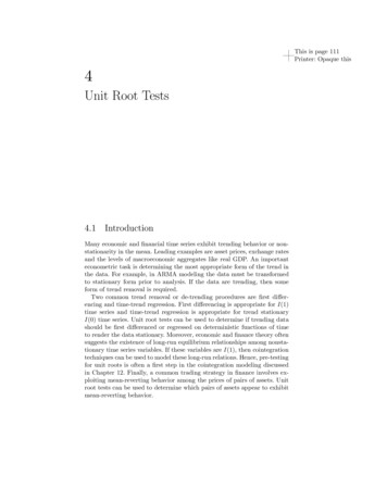
1164. Unit Root Tests4.3.1 Simulating the DF and Normalized Bias DistributionsAs mentioned above, the DF and normalized bias distributions must be obtained by simulation methods. To illustrate, the following S-PLUS functionwiener produces one random draw from the functions of Brownian motionthat appear in the limiting distributions of tφ 1 and T (φ̂ 1):wiener function(nobs) {e rnorm(nobs)y cumsum(e)ym1 y[1:(nobs-1)]intW2 nobs (-2) * sum(ym1 2)intWdW nobs (-1) * sum(ym1*e[2:nobs])ans list(intW2 intW2,intWdW intWdW)ans}A simple loop then produces the simulated distributions: }nobs 1000nsim 1000NB rep(0,nsim)DF rep(0,nsim)for (i in 1:nsim) {BN.moments wiener(nobs)NB[i] BN.moments intWdW/BN.moments intW2DF[i] BN.moments intWdW/sqrt(BN.moments intW2)Figure 4.2 shows the histograms and density estimates of the simulateddistributions. The DF density is slightly left-skewed relative to the standardnormal, and the normalized bias density is highly left skewed and nonnormal. Since the alternative is one-sided, the test statistics reject if theyare sufficiently negative. For the DF and normalized bias densities theempirical 1%, 5% and 10% quantiles are quantile(DF,probs c(0.01,0.05,0.1))1%5%10%-2.451 -1.992 -1.603 quantile(NB,probs c(0.01,0.05,0.1))1%5%10%-11.94 -8.56 -5.641For comparison purposes, note that the 5% quantile from the standardnormal distribution is -1.645.The simulation of critical values and p-values from (4.1) and (4.2) isstraightforward but time consuming. The punitroot and qunitroot func-

4.3 Autoregressive Unit Root TestsSimulated normalized bias0050100100200150300200Simulated DF E 4.2. Histograms of simulated DF and normalized bias distributions.tions in S FinMetrics produce p-values and quantiles of the DF and normalized bias distributions based on MacKinnon’s (1996) response surfacemethodology. The advantage of the response surface methodology is thataccurate p-values and quantiles appropriate for a given sample size can beproduced. For example, the 1%, 5% and 10% quantiles for (4.2) and (4.1)based on a sample size of 100 are qunitroot(c(0.01,0.05,0.10), trend "nc", statistic "t", n.sample 100)[1] -2.588 -1.944 -1.615 qunitroot(c(0.01,0.05,0.10), trend "nc", statistic "n", n.sample 100)[1] -13.086 -7.787 -5.565The argument trend "nc" specifies that no constant is included in thetest regression. Other valid options are trend "c" for constant only andtrend "ct" for constant and trend. These trend cases are explained below. To specify the normalized bias distribution, set statistic "n". Forasymptotic quantiles set n.sample 0.Similarly, the p-value of -1.645 based on the DF distribution for a samplesize of 100 is computed as punitroot(-1.645, trend "nc", statistic "t")[1] 0.0945

1184. Unit Root TestsCase I: I(0) data-52406581010Case I: I(1) data050100150200250050150200250200250Case II: I(0) data055101015152020252530Case II: I(1) data100050100150200250050100150FIGURE 4.3. Simulated I(1) and I(0) data under trend cases I and II.4.3.2 Trend CasesWhen testing for unit roots, it is crucial to specify the null and alternativehypotheses appropriately to characterize the trend properties of the dataat hand. For example, if the observed data does not exhibit an increasingor decreasing trend, then the appropriate null and alternative hypothesesshould reflect this. The trend properties of the data under the alternativehypothesis will determine the form of the test regression used. Furthermore, the type of deterministic terms in the test regression will influencethe asymptotic distributions of the unit root test statistics. The two mostcommon trend cases are summarized below and illustrated in Figure 4.3.Case I: Constant OnlyThe test regression isyt c φyt 1 εtand includes a constant to capture the nonzero mean under the alternative.The hypotheses to be tested areH0H1: φ 1 yt I(1) without drift: φ 1 yt I(0) with nonzero meanThis formulation is appropriate for non-trending financial series like interestrates, exchange rates, and spreads. The test statistics tφ 1 and T (φ̂ 1)