WIXLIB

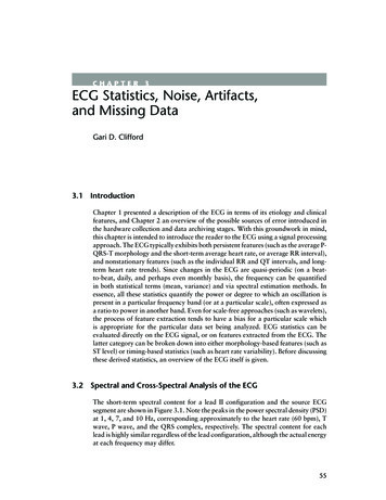
P1: ShashiAugust 24, 200611:39Chan-HorizonAzuaje Book3.3 Standard Clinical ECG Features61Figure 3.6 Standard fiducial points in the ECG (P, Q, R, S, T, and U) together with clinical features(listed in Table 3.1).either reduce noise or average out short-term beat-to-beat interval-related changes.The complex heart rate-related changes in the ECG morphology (such as QThysteresis4 ) can themselves be indicative of problems. However, a clinician canextract enough diagnostic information to make a useful assessment of cardiac abnormality from just a few simple measurements.Figure 3.6 illustrates the most common clinical features, and Table 3.1 illustratestypical normal values for these standard clinical ECG features in healthy adult malesin sinus rhythm, together with their upper and lower limits of normality. Note thatthese figures are given for a particular heart rate. It should also be noted that theheart rate is calculated as the number of P-QRS-T complexes per minute, but isoften calculated over shorter segments of 15 and sometimes 30 seconds. In termsof modeling we can think of this heart rate as our operating point around whichthe local interbeat interval rises and falls. Of course, we can calculate a heart rateover any scale, up to a single beat. In the latter case, the heart rate is termed theinstantaneous (or beat-to-beat) heart rate, HRi 60/RRn , of the nth beat. Eachconsecutive beat-to-beat, or RR, interval5 will be of a different length (unless thepatient is paced), and a correlated change in ECG morphology is seen on a beat-tobeat basis.4.5.See Section 3.4 and Chapter 11.The beat-to-beat interval is usually measured between consecutive R-peaks and hence termed the RRinterval. See Section 3.7.

P1: ShashiAugust 24, 200611:39Chan-HorizonAzuaje Book62ECG Statistics, Noise, Artifacts, and Missing DataTable 3.1 Typical Lead II ECG Features and Their Normal Values in SinusRhythm at a Heart Rate of 60 bpm for a Healthy Male Adult (see text andFigure 3.6 for definitions of intervals)FeatureP widthPQ/PR intervalQRS widthQTc intervalP amplitudeQRS heightST levelT amplitudeNormal Value110 ms160 ms100 ms400 ms0.15 mV1.5 mV0 mV0.3 mVNormal Limit 20 ms 40 ms 20 ms 40 ms 0.05 mV 0.5 mV 0.1 mV 0.2 mVNote: There is some variation between lead configurations. Heart rate, respirationpatterns, drugs, gender, diseases, and ANS activity also change the values. QTc αQT1where α (RR) 2 . About 95% of (normal healthy adult) people have a QTc between360 ms and 440 ms. Female durations tend to be approximately 1% to 5% shorterexcept for the QT/QTc, which tends to be approximately 3% to 6% longer than formales. Intervals tend to elongate with age, at a rate of approximately 10% per decadefor healthy adults.Often, the RR interval will oscillate periodically, shortening with inspiration(and lengthening with expiration). This phenomenon, known as respiratory sinusarrhythmia (RSA) is partly due to the Bainbridge reflex, the expansion and contraction of the lungs and the cardiac filling volume caused by variations of intrathoracic pressure [9]. During inspiration, the pressure within the thorax decreases andvenous return increases, which stretches the right atrium resulting in a reflex thatincreases the local heart rate (i.e., shortens the RR intervals). During expiration, thereverse of this process results in a slowing of the local heart rate. In general, thenormal beat-to-beat changes in morphology are ignored, except for derivationsof respiration, although the phase between the respiratory RR interval oscillations and respiratory-related changes in ECG morphology is not static; see Section3.8.2.2 and Chapter 8. The reason for this is that the mechanisms which alter amplitude and timing on the ECG are not exactly the same (although they are coupledeither mechanically or neurally with a phase delay which may change from beat tobeat; see Chapter 8). Changes in the features in Table 3.1 and Figure 3.6, therefore,occur on a beat-to-beat basis as well as because of shifts in the operating point(average heart rate), although this is a second order effect.The PR interval extends from the start of the P wave to the end of the PQjunction at the very start of the QRS complex (that is, to the start of the R or Qwave). Therefore, this interval is sometimes known as the PQ interval. This intervalrepresents the time required for the electrical impulse to travel from the SA nodeto the ventricle and normal values range between 120 and 200 ms. The PR intervalhas been shown to lengthen and shorten with respiration in a similar manner to theRR interval, but is less pronounced and is not fully correlated with the RR intervaloscillations [10].The global point of reference for the ECG’s amplitude is the isoelectric level,measured over the short period on the ECG between the atrial depolarization(P wave) and the ventricular depolarization (QRS complex). In general, this pointis thought to be the most stable marker of 0V for the surface ECG since there isa short pause before the current is conducted between the atria and the ventricles.

P1: ShashiAugust 24, 200611:39Chan-HorizonAzuaje Book3.3 Standard Clinical ECG Features63Interbeat segments are not usually used as a reference point because activity beforethe P wave can often be dominated by preceding T-wave activity.The QRS width is representative of the time for the ventricles to depolarize,typically lasting 80 to 120 ms. The lower the heart rate, the wider the QRS complex, due to decreases in conduction speed through the ventricle. The QRS widthalso changes from beat-to-beat based upon the QRS axis (see Chapter 1), which iscorrelated with the phase of respiration (see Chapter 8) and with changes in RRinterval and therefore the local heart rate. The RS segment of the QRS complexis known as the ventricular activation time (VAT) and is usually shorter (lastingaround 40 ms) than the QR segment. This asymmetry in the QRS complex is nota constant and varies based upon changes in the autonomic nervous system (ANS)axis, lead position, respiration and heart rate (see Chapter 8).The QRS complex usually rises (for positive leads) or falls to about 1 to 2 mVfrom the isoelectric line for normal beats. Artifacts (such as electrode movements)and abnormal beats (such as ventricular ectopic beats) can be several times larger inamplitude. In particular, baseline wander can often be the largest amplitude signalon the ECG, with the QRS complexes appearing as almost indistinguishable periodicanomalies. For this reason, it is important to allow sufficient dynamic range in theamplification (or digital storage) of ECG data; see Chapter 2.The point of inflection after the S wave is known as the j-point, and is often usedto define the beginning of the ST segment. In normals, it is expected to be isoelectricsince it is the pause between ventricular depolarization and repolarization. The STlevel is generally measured around 60 to 80 ms after the j-point, with adjustments forlocal heart rates (see Chapters 9 and 10). Abnormal changes in the ECG, defined bythe Sheffield criteria [11], are ST level shifts 0.1 mV (or about 5% to 10% of theQRS amplitude for a sinus beat on a V5 lead). Since only small deviations form theisoelectric level are significant markers of cardiac abnormality (such as ischemia),the correct measurement of the isoelectric line is crucial. The interbeat segments between the end of the P wave and start of the Q wave are so short (less than 10 samplesat 125 Hz), that the isoelectric baseline measurement is prone to noise. Multiple-beataveraging is therefore often employed. ST segment and j-point elevation, commonin athletes, has been reported to normalize with exercise [12] and therefore j-pointelevations may be difficult to distinguish from other changes seen in ECG.The QT interval is measured between the onset of the QRS complex and the endof the T wave. It is considered to represent the time between the start of ventriculardepolarization and the end of ventricular repolarization and is therefore useful asa measure of the duration of repolarization (see Chapter 11). The QT interval variesdepending on heart rate, age, and gender. As with some other parameters in the ECG,it is possible to approximate the (average) heart rate dependency of the QT intervalˆ is the local average RR interval.ˆ 12 where RRby multiplying it by a factor α ( RR)The resultant QT interval is called the corrected QT interval, QTc [13]. However,this factor works over a limited range and is subject dependent to some degree, overand above the usual confounding variables of age, gender, and drug regime; seeSection 3.4.1.Furthermore, ANS activity shifts can also change α. In general, the last RRinterval duration affects the action potential (see Chapter 1) and hence the QTinterval. It is also known that the QT-RR dependence is both a function of the

P1: ShashiAugust 24, 200611:39Chan-HorizonAzuaje Book64ECG Statistics, Noise, Artifacts, and Missing Dataaverage heart rate and the instantaneous interval, RRi [14]. Note that there issome variation in these parameters between lead configurations. Although interlead differences are sometimes used as cardiovascular markers themselves (such asin QT dispersion [15]), it is unclear whether there is a specific physiological originto such differences, or whether such metrics are just measuring an artifact whichcorrelates with a clinical marker [16, 17].One of the problems in measuring the QT interval correctly (apart from thenoise in the ECG and the resultant onset and offset ambiguities) is due to thechanges in the j-point and T wave morphology with heart rate. It has been observedthat as the heart rate increases, the T wave increases in height and becomes moresymmetrical [18]. Furthermore, in some subject groups (such as athletes), the Twave is often observed to be inverted [12].To summarize, the following changes are typically observed with increasingheart rate [12, 18, 19]: The average RR interval decreases.The PR segment shortens and slopes downward (in the inferior leads).The P wave height increases.The Q wave becomes slightly more negative (at very high heart rates).The QRS width decreases.The R wave amplitude decreases in the lateral leads (e.g., V5) at and just afterhigh heart rates.The S wave becomes more negative in the lateral and vertical leads (e.g., V5and aVF). As the R wave decreases in amplitude, the S wave increases in depth.The j-point often becomes depressed in lateral leads. However, subjects witha normal or resting j-point elevation may develop an isoelectric j-point withhigher heart rates.The ST level changes (depressed in inferior leads).The T wave amplitude increases and becomes more symmetrical (although itcan initially drop at the onset of a heart rate increase).The QT interval shortens (depending on the autonomic tone).The U wave does appear to change significantly. However, U waves may bedifficult to identify due to the short interval between the T and followingbeat’s P waves at high heart rates.It should be noted however, that this simple description is insufficient to describethe complex changes that take place in the ECG as the heart rate increases anddecreases. These dynamics are further explored in the following section.3.4 Nonstationarities in the ECGNonstationarities in the ECG manifest both in an interbeat basis (as RR intervaltiming changes) and on an intrabeat basis (as morphological changes). Althoughthe former changes are often thought of as rhythm disturbances and the latteras beat abnormalities, the etiology of the changes are often intricately connected.To be clear, although we could categorize the beat-to-beat changes in the RR interval

P1: ShashiAugust 24, 200611:39Chan-HorizonAzuaje Book3.4 Nonstationarities in the ECG65timing and ECG morphology as nonstationary, they can actually be well representedby nonlinear models (see Section 3.7 and Chapter 4). This chapter therefore refersto these changes as stationary (but nonlinear). The transitions between rhythms is anonstationary process (although some nonlinear models exist for limited changes).In this chapter, abnormal changes in beat morphology or rhythm that suggest arapid change in the underlying physiology are referred to as nonstationary.3.4.1Heart Rate HysteresisSo far we have not considered the dynamic effects of heart rate on the ECG morphology. Sympathetic or parasympathetic changes in the ANS which lead to changes inthe heart rate and ECG morphology are asymmetric. That is, the dynamic changesthat occur as the heart rate increases, are not matched (in a time symmetric manner)when the heart rate reduces and there is a (several beat) lag in the response betweenthe RR interval change and the subsequent morphology change. One well-knownform of heart rate-related hysteresis is that of QT hysteresis. In the context of QTinterval changes, this means that the standard QT interval correction factors6 are agross simplification of the relationship, and that a more dynamic model is required.Furthermore, it has been shown that the relationship between the QT and RR interval is highly individual-specific [20], perhaps because of the dynamic nature ofthe system. In the QT-RR phase plane, the trajectory is therefore not confined to asingle line and hysteresis is observed. That is, changes in RR interval do not causeimmediate changes in the QT interval and ellipsoid-like trajectories manifest in theQT-RR plane. Figure 3.7 illustrates this point, with each of the central contoursindicating a response of either tachycardia (RT) and bradycardia (RB) or normalresting. From the top right of each contour, moving counterclockwise (or anticlockwise); as the heart rate increases (the RR interval drops) the QT interval remainsconstant for a few beats, and then begins to shorten, approximately in an inversesquare manner. When the heart rate drops (RR interval lengthens) a similar timedelay is observed before the QT interval begins to lengthen and the subject returnsto approximately the original point in the QT-RR phase plane. The difference between the two trajectories (caused by RR acceleration and deceleration) is the QThysteresis, and depends not only on the individual’s physiological condition, butalso on the specific activity in the ANS. Although the central contour defines thelimits of normality for a resting subject, active subjects exhibit an extended QT-RRcontour. The 95% limits of normal activity are defined by the large, asymmetricdotted contour, and activity outside of this region can be considered abnormal.The standard QT-RR relationship for low heart rates (defined by the Fridericiacorrection factor QTc QT/RR1/3 ) is shown by the line cutting the phase planefrom lower left to upper right. It can be seen that this factor, when applied tothe resting QT-RR interval relationship, overcorrects the dynamic responses in thenormal range (illustrated by the striped area above the correction line and belowthe normal dynamic range) or underestimates QT prolongation at low heart rates6. Many QT correction factors have been considered that improve upon Bazett’s formula (QTc QT/ RR),including linear regression fitting (QTc QT 0.154(1 RR)), which works well at high heart rates, andthe Fridericia correction (QTc QT/RR1/3 ), which works well at low heart rates.

P1: ShashiAugust 24, 200611:39Chan-Horizon66Azuaje BookECG Statistics, Noise, Artifacts, and Missing DataFigure 3.7 Normal dynamic QT-RR interval relationship (dotted-line forming asymmetric contour)encompasses autonomic reflex responses such as tachycardia (RT) and bradycardia (RB) with hysteresis. The statistical outer boundary of the normal contour is defined as the upper 95% confidencebounds. The Fridericia correction factor applied to the resting QT-RR interval relationship overcorrects dynamic responses in the normal range (striped area above correction line and below 95%confidence bounds) or underestimates QT prolongation at slow heart rates (shaded area above 95%confidence bounds but below Fridericia correction). QT prolongation of undefined arrhythmogenicrisk (dark shaded area) occurs when exceeding the 95% confidence bounds of QT intervals duringunstressed autonomic influence. (From: [21]. c 2005 ASPET: American Society for Pharmacologyand Experimental Therapeutics. Reprinted with permission.)(shaded area above normal range but below Fridericia correction) [21]. AbnormalQT prolongation is illustrated by the upper dark shaded area, and is defined to bewhen the QT-RR vector exceeds the 95% normal boundary (dotted line) duringunstressed autonomic influence [21].Another, more recently documented heart rate-related hysteresis is that of ST/HR[22], which is a measure of the ischemic reaction of the heart to exercise. If ST depression is plotted vertically so that negative values represent ST elevation, andheart rate is plotted along the horizontal axis typical ST/HR diagrams for a clinically normal subject display a negative hysteresis in ST depression against HR,(a clockwise hysteresis loop in the ST-HR phase plane during postexercise recovery).Coronary artery disease patients, on the other hand, display a positive hysteresisin ST depression against HR (a counterclockwise movement in the hysteresis loopduring recovery) [23].It is also known that the PR interval changes with heart rate, exhibiting a(mostly) respiration-modulated dynamic, similar to (but not as strong as) the modulation observed in the associated RR interval sequence [24]. This activity is describedin more detail in Section 3.7.3.4.2ArrhythmiasThe normal nonstationary changes are induced, in part, by changes in the sympathetic and parasympathetic branches of the autonomic nervous system. However,

P1: ShashiAugust 24, 200611:39Chan-HorizonAzuaje Book3.5 Arrhythmia Detection67sudden (abnormal) changes in the ECG can occur as a result of malfunctions in thenormal conduction pathways of the heart. These disturbances manifest on the ECGas, sometimes subtle, and sometimes gross distortions of the normal beat (dependingon the observation lead or the physiological origin of the abnormality). Such beatsare traditionally labeled by their etiology, into ventricular beats, supraventricularand atrial.7Since ventricular beats are due to the excitation of the ventricles before the atria,the P wave is absent or obscured. The QRS complex also broadens significantly sinceconduction through the myocardium is consequently slowed (see Chapter 1). Theoverall amplitude and duration (energy) of such a beat is thus generally higher. QRSdetectors can easily pick up such high energy beats and the distinct differences inmorphology make classifying such beats a fairly straightforward task. Furthermore,ventricular beats usually occur much earlier or later than one would expect for anormal sinus beat and are therefore known as VEBs, ventricular ectopic beats (fromthe Greek, meaning out of place).Abnormal atrial beats exhibit more subtle changes in morphology than ventricular beats, often resulting in a reduced or absent P wave. The significant changes foran atrial beat come from the differences in interbeat timings (see Section 3.2.2). Unfortunately, from a classification point of view, abnormal beats are sometimes morefrequent when artifact increases (such as during stress tests).

August 24, 2006 11:39 Chan-Horizon Azuaje Book 3.2 Spectral and Cross-Spectral Analysis of the ECG 57 Figure 3.2 PSD (dB/Hz) of all 12 standard leads of 10 seconds of an ECG in sinu