Transcription
CS-BIGS 4(1): 9-22 2010 g2.pdfDynamic Data VisualizationChamont WangThe College of New Jersey, USAMichele MeisnerThe College of New Jersey, USAIn this article, we use four examples to illustrate a variety of techniques for the visualization of complicated data sets.The examples include business data, storm tracking, New Jersey Department of Education records, and classroomobservations. The techniques are used to deal with certain geo-spatial patterns and cross-tabulations on the fly. Videoclips are referenced throughout to illustrate the interactivity, kinetic actions, and animations of these approaches. Thearticle contains no math and is accessible to all statistics users, including students in high-school AP Stat classes.Key Words: Data Visualization, Geographic Patterns, Google Map, Cross-TabulationsIntroductionModern data analysis often involves complicated datastructures with multi-years, multi-categories, multigeographic-regions, and layered cross-tabulations.Moreover, the data may change at an ever-increasingspeed. For this kind of situation, traditional tools andcode-writing may not be the best way to extract usefulinformation out of a complicated data set.In recent years, books and software packages have pickedup the pace to provide users with new platforms fordynamic data visualization. A Google search on “datavisualization” leads to 1,220,000 links. Examples that welike include JMP, RapidNet, Gephi, Perceptual Edge, toname a few.In this article, we will present examples to illustrate theadvantages and limitations of two different visualizationtechnologies and show how to use the two tocomplement each other. The first is called Tableau andthe second is Statistica. The reasons for this choice areas follows:1. Students or anyone with basic statistical backgroundcan start using the tools after a single lab session.2. The tools can handle complicated data sets rapidly.3. Both are full of sophisticated techniques to challengestudents. There are indeed countless directions to gowhen the user reaches the Jedi level.4. Both come with a wide array of sample workbookswith the raw data included.5. They promote the journey from Data to StoryTelling.6. In spite of their sophistication and advanced features,the guiding philosophy of these technologies is thesimplicity of data visualization. This philosophyembodies what Albert Einstein said, “Everythingshould be made as simple as possible, but notsimpler.” It also echoes the da Vinci quote:“Simplicity is the ultimate sophistication.”
10 Dynamic Data Visualization / Wang & MeisnerWe believe such a philosophy should permeate all phasesof data visualization.For data visualization, Tableau has further advantages:1. It handles Geographic data with a few clicks of themouse.2. In addition, it provides a quick, clever link to GoogleEarth technology.3. It is free for academic use.4. It zooms in on any specific part of the data and thenexports it for external use with great ease.5. It uses a Dashboard technology to summarize keyfindings.The creator of Tableau is a Stanford professor, PatHanrahan, who worked for a Defense Department projectaiming at increasing people's ability to analyzeinformation. He is a founding member of Pixar, thestudio that made the animated films such as Toy Storyand Wall-E (http://www.pixar.com/). His team comprisessome of the best minds in the industry.In our experience, the new technologies sharpen theuser’s mind on the intricacies of the data rather thantaking the user’s focus off the data as one oftenencounters when using traditional tools. In this article,we will present a number of examples to illustrate thepower of these tools. The examples, on the other hand,should not be taken as the equivalence of the full power(or even a fraction) of what the new technologies canaccomplish.Example 1 (Super-Store Sales Data)This data set has 26 columns and 8,400 rows; it is one ofTableau’s sample workbooks and free data sets. Theirsample workbook provides certain insights of the data;our analysis will venture into a different direction. Tobegin with, the variables in this data include Customer NameCustomer Segment (Small Business, Corporate,Home Office, etc.)Customer State (New York, Ohio, Michigan, etc.)Product 1 – Category (Office Supplies, Technology,etc.)Sales VolumeProfitDiscountOthersThis data set holds a lot of information about a specificcompany. Our goal is to dig deeper into some of thesevariables to decipher how well the company is doing andin which sales categories and geographic locations thiscompany needs to improve.To proceed, our first question was: What can we do withthis data set? A few possibilities are as follows: Association Rule which is common in data mining;e.g., ID Customer id; Target Product.Companies such as Amazon.com, Walmart.com andcountless others use Association Rule to great effect.Predictive modeling: Decision Tree, Regression,Neural Network, etc. (e.g., Target profit,Predictors: sale, discounts, regions, categories, etc.).Data Visualization.In this article, we focus on data visualization. Inparticular, we will throw a series of questions and thenrespond with rapid-fire answers. The answers below arestatic; to see them in action, please visit the links below:http://www.youtube.com/watch?v CdjuKww1zQ8 andhttp://www.youtube.com/watch?v BF1WLgBY3K4 forYouTube video clips. The video clips are also posted withthis article on the journal web site.This example is very useful for business applications andwill be unfolded in the following manner: What is the company’s bottom line within eachproduct category and sub-category?What kinds of products sell well but are notprofitable?How can geographic information be used to pinpointthe region where certain products are not profitable?Drill down on geographic and calendar information:For states like New Jersey, which year is leastprofitable? And in which part of New Jersey is thecompany not doing well?We now proceed to answer the above questions intandem:1. A key issue about how a company is doing would be:what is the sales volume?In our video, one can see how in a few seconds, weproduced the following chart:Figure 1.1. Sales Volume.
11 Dynamic Data Visualization / Wang & MeisnerSo the total sales is about 15 million. That is a largeamount of money, and a thorough analysis of thedata may be worthwhile. For instance, the chartshows that Technology accounts for almost 6million of the sales, and a more detailed analysis mayprovide information to help improve sales.2. Our next question is: what is the sales volume ineach product category?Figure 1.4. Profit by Region.Figure 1.2. Sales Volumes for 3 Different Products.In Table 1.2, the portion circled in red is called ashelf in Tableau. A drag of the variable, Sales, to theText shelf immediately gives the exact numbers ofthe sales in each category. The separation in thisplot makes it easier to see the exact sales volumes ofthe three categories.3.Note that high sales volume does notguarantee high profit. Hence our next question is:Which category is most profitable? We see thatFurniture sells well, but is not profitable:Figure 1.5. Profit by State.The chart shows that New Jersey loses a lot of moneyon furniture, and Connecticut is in a similar situation.Note that we used the Filters tab to select only thefew States of interest. Again, by point-and-click, thisis done in about 15 seconds.6. Calendar information: The data containinformation for years 2006, 2007, 2008 and 2009. Soour next question is: for states such as New Jersey,which year is least profitable?Figure 1.3. Profit vs. Sales for 3 Different Products.4. Geographic information: In real estate, the threemost important variables are: location, location, andlocation. This is probably the same with many otherbusiness applications. For this study, we can usegeographic information to pinpoint the region wherefurniture is not profitable. East (NY, NJ, )? West(California, .)? Central? Or South? Figure 1.4shows that furniture is losing money in the East.Note that in Figure 1.4, a Title and Caption havebeen added to the chart for future reference. Thesefeatures aid in showing the complete picture andorganizing your thoughts.5. Drill down: we now examine the geographicinformation in more details in an attempt to seewhich State in the East is least profitable.Figure 1.6. Profit by Year and by State.The chart says that New Jersey lost about 9,500 in2006, lost even more in 2008, but did better in 2009.7. Map: The above analyses used only bar charts. Wenow add a new dimension by using a map to seewhich part of New Jersey is not doing well. Theanswer to this question requires only a few clicks and
12 Dynamic Data Visualization / Wang & Meisnerdrag-and-drops. We double click on Longitude andLatitude to bring up the map.Figure 1.9. Profit Map near Princeton Area.Figure 1.7. Profit Map.This mapping technique can be used with any dataset that has zip code, county information, or numericvalues of latitude and longitude variables.Themapping does not require internet access, but theonline version of Tableau provides additional mapoptions.The chart shows that the Princeton location is doingwell and making a profit of 21,245 over the studyperiod.9. Drill down-II: Finally, we want to know what typesof furniture are not profitable.In Figure 1.7, if we zoom in on New Jersey, a big reddot will appear in northen Jersey. In addition we canmodify the map to show the progression throughmultiple years. Hovering the mouse on the dotdisplays the zip code information as shown in thenext chart.Figure 1.10. Drill Down: Profit of Sub-category.The chart shows that Bookcases and Tables are moneylosers. Nevertheless, it may be worthwhile to keep themin stock to help bring in customers for other items.In conclusion, this case study shows that with the help ofmodern visualization tools, bar charts alone can be usedto extract information rapidly from files with acomplicated data structure. For this specific data set, onecan easily obtain the following information:Figure 1.8. Geo-spatial Display of Profit in New Jerseyin Different Years.By moving the mouse over that specific location(zipcode 07514, which is Paterson, NJ), one cansee that the store lost about 7,200 in 2006 but brokeeven in 2009.8. A specific question is: how is the store in Princetonarea performing? Drill down to specific year, month, region and subregion.Pinpoint the regions that are in the red.View the above information in a calender sequence,either one period a time or multiple periods on adashboard.In addition to the dynamic use of Bar Charts, modernvisualization tools allow the user to view geographicinformation with only a few clicks of the mouse. This is aleap from a book with words to a map with charts. A
13 Dynamic Data Visualization / Wang & Meisnerfurther leap is to add calender information on the map,leading to a geo-spatial display for a broad view ofmultiple variables on different regions in different timeperiods.For this data set, our focus is on sales volumn and profit.Other variables such as Discount, can also provide veryuseful insight of the data. See the following site for aspirited presentation that uses this variableeffectively: le 2 (Storm Tracking and Animation)This data set has 16 columns and 572 rows. It wasadapted from a Tableau sample workbook. Their staticchart led us to modifications and animations in thisstudy. The variables in the data include Storm Name (ALEX, BONNIE, DANIELLE, etc.)Storm speed (mph)Wind speed (kt; 1 knot 1.852km/hr 1.151miles/hr)Pressure (mb; 1 millibar (1/1000) bar; 1 barcorresponds to the atmospheric pressure on earth atsea level)Longitude (deg)Latitude (deg)DateOthersIn this example, we will investigate the relationshipsbetween Wind Speed, Storm speed, and Pressure. Sincethe data includes Latitude, Longitude, and Date, we canalso perform an animation of storm movements.Interestingly, when we performed this animation in class,a student gushed and asked the following question: “Isthis what they do on the Weather Channel?”To perform the storm tracking, we double click onLongitude and Latitude respectively to activate the map.Adding Color (Storm Name), Text (Storm Name), Size(Storm Speed), and Filtering out a few storms make themap easier to read.To animate the storm tracking, we drag Date to thePages shelf, change the Date from Year to Day, thenclick on the Play button to see the storms in motion.The speed of the animation can be adjusted if needed. om/watch?v -muHR6lHbko(5:17 minutes), and is posted with the article on thejournal website.Figure 2.1. Storm Tracking.Figure 2.1 shows the following: During the same length of time, Karl traveled veryfar, while Jeanne stayed within a more confined area.The size of the dots reflects the Wind Speed of thestorm. Karl gained a lot of strength early on andthen remained a strong force for a very long distanceon the sea.Jeanne, on the other hand, gained a lot of power inthe middle of the course, maintained its strengthuntil hitting Florida, and then weakenedsubstantially on the mainland.Karl and Lisa did not threaten people on land, whileJeanne might have caused severe damage to lives andproperties.A potential application of the above technique is theanimation of Bubble graphs. A Google image search ofBubble plot yielded 453,000 charts. It may be possible torelease some of these bubbles in sequence if the timestamp is available in the data.Next we will examine six (6) variables on a histogram.To begin with, we high-light Wind Speed and click onthe Show Me button to activate the plain histogram:
14 Dynamic Data Visualization / Wang & Meisnerthe thin bars are a little misleading. A related issue of thebar size will be discussed after Figure 2.5.Now we add Storm Name to the Text shelf:Figure 2.2. Histogram of Wind Speed.Here we can see that a wind speed of 30 corresponds tothe highest count of wind speed, and as the wind speedbecomes greater than the 30 peak, the count drops.To view more variables in this same chart we addPressure to the Size shelf, and add Storm Speed to theColor shelf:Figure 2.4. Histogram Wind Speed;Color Storm Speed; Size Pressure; Text Storm Name.Figure 2.4 is hard to read on a printing medium such as apiece of paper or a pdf file. As a result, we use the Filteroption to focus on three storms (Jeanne, Lisa, and Karl)that were shown on Figure 2.1:Figure 2.3. Histogram Wind Speed;Color Storm Speed; Size Pressure.Here the width of each bar shows the pressure and thecolor represents the storm speed. The wind speed of 30,which had the highest wind speed count, alsocorresponds to the greatest pressure (thickest bar) andthe highest storm speed (darkest red color). Studentswho saw this chart tend to conclude that in general, windspeed, storm speed, and pressure are correlated. In thesubsequent analysis, we will discuss this issue in moredepth.Another observation is that storms with a wind speed of10 and 130 seem to have very similar pressures (as seenby the similar widths). The qeustion arises of why theywould have the same pressure. Hovering the mouse tothe bars would reveal that the pressure is 1998 mb at theleft end and 7385 mb when the Wind Speed is 130. SoFigure 2.5. Histograms of Jeanne, Lisa, and Karl.The chart shows that the Wind Speeds (x-axis) of Lisa donot go beyond 60 kt. In contrast, the Wind Speeds ofJeanne and Karl may reach 100 kt or more.Onequestion would be the overall relationships betweenWind Speed, Storm Speed and Pressure. For this task,we will use different techniques in the subsequentdiscussions.The trade-off between Figures 2.4 and 2.5 is that the firstchart provides more information (6 variables for each ofthe 15 storms) while the other is easier to understand (5variables for each of the 3 storms). To view the details ofeach square, we simply hover the mouse to the box.Furthermore, one can add the sixth variable Date to the
15 Dynamic Data Visualization / Wang & MeisnerPages shelf and flip the pages to see how the Histogramevolves with time.and should be able to yield more insights in countlessother studies.Note that the legend of the Histogram says that the sizeof the bar is determined by the Sum of the Pressure. Youcan easily change the Sum of Pressure to the Average ofPressure (which ranges from 917 to 1008 mb). As aresult, the difference of the bar sizes would be so smallthat the chart would not be as appealing. A purpose ofour Figures 2.3-2.5 is to show the versality of the chart, sothe more interesting visual was used; the true utility ofusing the bar size may be realized in other studies.The next chart (Matrix Plot) shows the scatterplots ofWind Speed, Storm Speed, and Pressure. On thediagonal of the matrix, the histograms of the 3 variablesshow the following:Next we examine the relationship between Wind Speedand Storm Speed: Storm Speed is skewed to the right (with few stormsmoving at high speed),Wind Speed is also skewed to the right but not asseverely as Storm Speed, andPressure is skewed to the left, contrary to WindSpeed and Storm Speed.Figure 2.6. Wind Speed vs. Storm Speed: no pattern in thescatterplot.The scatterplot appears boring and does not reveal anyrelationship between the two variables. To brighten upthe dull scatterplot, first we add Storm Name to theColor and Text shelves and then add Trend Lines toproduce the following chart:Figure 2.8. Wind Speed, Storm Speed, and Pressure:Histograms and Scatterplots.The scatterplots, on the other hand, show the following: In general, Storm Speed is not correlated to WindSpeed or Pressure.Wind Speed and Pressure are negatively correlated.This is consistent with meteorological observationsthat tropical cyclones generally occur in areas of lowatmospheric pressure, with the lowest pressuresrecorded at the centers of the cyclones.The raw data is available at the following site; the sitealso provides other ways to visualize this particular dataset: torm-tracking.Figure 2.7. Wind Speed vs. Storm Speed; Color StormNames.The chart shows that for Karl, Wind Speed and StormSpeed are negatively correlated, while for Lisa, it is theopposite. This technique has been around for decades,Example 3 (Educational data)In this example, we used data from the website of NewJersey Department of
16 Dynamic Data Visualization / Wang & MeisnerEducation: http://www.state.nj.us/education/data/. Thevariables include School DistrictBudgetGraduation RateDropout RateDateOthersFirst, we tried to examine the Dropout Rate, and weproduced the following chart:Figure 3.3. Dropout Rates vs. Average Spending perStudent.The conventional way of dealing with scatterplots likethe ones in Figure 3.3 is to fit a regression line. But thiswould not be helpful. Instead, we add median lines onboth the x-axis and the y-axis (Color District; Text District):Figure 3.1. Dropout Rates of All Counties.In Figure 3.1, the horizontal axis is academic year, andthe vertical axis is the Dropout Rates of the Counties.The chart is hard to decipher, so we added District to thePages shelf and to the Text shelf. This is a veryimportant technique.Now the Pages can be flipped to see the dropout rates foreach district. For instance, the dropout rates at AtlanticCounty went downward, which is an improvement.However dropout rates at Ocean County, after someimprovements, went up significantly:Figure 3.2. Dropout Rates of Atlantic and Ocean Counties.The scatterplot below examines Dropout Rates againstAverage Spending per Student for the academic year 0607:Figure 3.4. Median Splits.The first quadrant shows the worst (names of the districtswith High Dropout Rates and High Spending), while thethird quadrant shows the best (names of the districts withLow Dropout Rates and Low Spending). Clearly certaindistricts have things to learn from others. In short, Figure3.4 identifies the following: the best districts, the worst,and the outlier, Cape May.In addition, note that the scatter-plot in Figure 3.4displays a total of 6 quantities: the two variables on theaxes, plus color and County names, plus the medians onthe x- and y-axes. Furthermore, we can view all detailedinformation by moving the mouse to a specific county.This is data visualization on the fly.Recall that Bar Charts can also display multiple variables(see Figure 2.4 with 5 variables on the chart). But ascatterplot can lock two specific variables on the chart toprovide a different way of stratification.
17 Dynamic Data Visualization / Wang & MeisnerThe next chart shows Graduation Rates against AverageSpending per Student. The Median Splits are used todecipher which districts have High Spending and LowGraduation rates.Figure 3.7. Average Spending per Student, by District.Figure 3.5. Graduation Rates vs. Average Spending perStudent.Now that we have two outliers: Cape May (Figure 3.5)and Mercer (Figure 3.7); the next chart (Figure 3.8)compares the two over a period of time from 1998 to2009.The second quadrant shows the best (districts with LowSpending and High Graduation), while the fourthquadrant shows the worst (districts with High Spendingand Low Graduation rates). The reasons for the LowGraduation Rates, however, are not clear from the data.On the chart, Cape May is an outlier: high spending andhigh graduation rate. Citizens in that county probablyare committed to good education regardless of the cost.The next chart shows that the overall Average Spendingper Student almost doubled over a ten-year period: 8,405 (in 1998) to 15,053 (2009).Figure 3.8. Cape May and Mercer.The chart indicates the following: the spending of CapeMay peaked in 06-07, after gradually increasing from1998, with a 25% jump from 05-06 to 06-07. It overtookMercer in 06-07 and 07-08, but Mercer went through theroof in 2008-2009. Cape May, on the other hand, cutback to a certain extent after the spending spree.We now summarize Figures 3.3 to 3.7 on a dashboard:Figure 3.6. Average Spending per Student, 1998-2009.Figure 3.6 appears to imply the trend of doubling forevery county. However, when we added District to theColor shelf, the chart shows that Mercer county is the bigspender in the last year of the study period.
18 Dynamic Data Visualization / Wang & MeisnerFigure 3.9. Dashboard of the NJ-DoE data.The top row displays plain graphs. The bottom rowdemonstrates that with a few clicks, modern visualizationtechniques can reveal a lot more information. Inaddition, the bottom row shows dropout rate, graduationrate, and average spending in one glance. The graphscomplement each other to provide decision makers abetter view of the overall situation.Finally, we double clicked on the Longitude and Latitudevariables to bring up a map. We then put the threevariables (Spending in the Color shelf, Graduation Ratein the Size shelf, and Dropout Rate in the Text shelf) ona map and then move the mouse to high-light any case(e.g., Atlantic county in Figure 3.10):Figure 3.11. Satellite Image.This technique can be useful in many real-worldscenarios. It can help with Campus Space Analysis,which may include the planning of campus construction,the management of campus wireless networks, andperhaps other novel applications.A different issuewould be the crime and security concerns on thecampuses. The U.S. Department of Education reportsthat campus crimes are occurring at surprisingly ty/crime/criminaloffenses/index.html). The crimes include AggravatedAssault, Arson, Burglary, Sex Offenses, Motor VehicleTheft, Murder, Manslaughter, and Robbery. In thecategory of Robbery alone, there were 11,659 cases in2001 and 9,367 cases in 2002.New technologies to fight against crimes are on the rise(see, e.g., Westphal, 2008). Examples in this regardinclude monitoring crime statistics by type, location, anda number of other criteria. Such applications are veryuseful in the fast-growing field of Fraud Detection, whichincludes the uncovering of Construction Fraud, MoneyLaundering, Alien Smuggling, Social Network Analysis,and Financial Transactions Investigation.Figure 3.10. Color Spending, Size Graduation, Text Dropout.The red box on the chart shows the exact Dropout rates,Graduation totals, and Spending at Atlantic county. Thenumbers may help administration on future planning.On the map, we right click on any location to find theoption of View Satellite Image which links Tableau mapsto Google maps.In Fraud Detection conferences that we have attended,quick links to Google Maps have generated considerableenthusiasm (see, e.g., i2 Intelligence-Led OperationsPlatform, p://www.i2group.com/us/news--events/events).We do believe that this new technology will be veryuseful in real-world crime fighting and fraud detection.Another application of the link to Google Maps is themonitoring of 911 calls for emergency responses to aspecific geographic location (medical assistance, assault,or fire related incidents). An example can be found inthe Tableau Wow sample workbook.
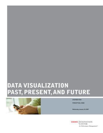
19 Dynamic Data Visualization / Wang & MeisnerTwo video clips for Example 3 can be foundat http://www.youtube.com/watch?v FQ4S 1KOffE, http://www.youtube.com/watch?v SHiEnIdUcuE, and areposted with this article on the journal website.Example 4 (Finding Patterns in the StudentExam Data)To begin with, we try to detect patterns by the use of a3D rotation graph. The action can be viewed in a shortvideo clip at http://www.youtube.com/watch?v Tg0Rdr3kiU (1:20 minutes). The default 3D graph and aversion of its rotation are in Figure 4.1 below. Examiningthe graphs, we ask the question: are there any patterns inthe data?In this example, we will explore a different technology thatis more in the mode of traditional statistical analysis. Thisapproach complements the technology in Examples 1-3 ofthis article. The tools we will use are part of the Statisticapackage. A rich array of examples in this category can befound at hniques/?button 2.The DataThe data in the following table contains the exam scoresof 19 students in an Introductory Statistics course at acollege:Exam 178655294379971854268499087987792509171Exam 199299580735361409589407296427584Figure 4.1. 3D rotation graphs of the Exam-Final data.In our classroom surveys, most students see no pattern inthe original depiction. After rotating the plot they noticea linear relationship in the second graph in Figure 4.1 butnot much else. A few see the outlier. After someexplanations, they see that in addition to the outlier,there are three clusters: top students, middle students,and failing students.In the hunt for failing students, we use a Statistical Lasso,which was inspired by the traditional Cowboy Lasso:Figure 4.2. Cowboy Lasso.For both lassos, the idea of capturing a target for a closerlook is the same:Given the data, one can build regression models toforecast the Final grade. In this article, however, we willfocus on the visualization aspects of the data. A total ofthree video clips are supplied to display the steps of thisapproach and are posted on the journal website:a) Pattern Detection in 3-D (1:20 minutes)http://www.youtube.com/watch?v Tg0R-dr3kiUb) Cowboy Lasso and Statistical Lasso ():57 minutes)http://www.youtube.com/watch?v ngetV0af Qcc) Icon Plots (2:32 minutes)http://www.youtube.com/watch?v llfdhurNrs8Figure 4.3. A Statistical Lasso.
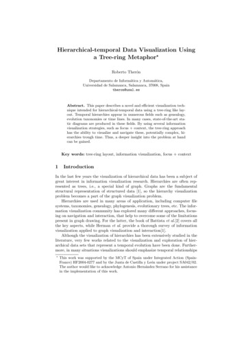
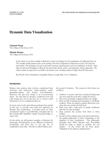
20 Dynamic Data Visualization / Wang & MeisnerThe hunt reveals that Students #3, 5, 9, 11, and 17 arefailing and need immediate attention. A video clip tocapturethisactionisavailableat http://www.youtube.com/watch?v ngetV0af Qc.Next we use a variety of Icon plots to investigate thestudents’ exam scores. The first of this kind is called Starplot:What happened was that Student #14 had learned somekind of Statistics from certain unknown places andindeed performed very well in Exam-1. Then he cutclasses, missed homework assignments, skipped groupmeetings, and got only 60 on Exam-2. The instructorintervened to no avail. By the time of the Final, thegrade of that student went down the drain.The story of Student #14, as shown in the Profile Plot,stands out from the other students as a straggler. Byusing the technique of Lasso, we can see again that theoutlier on the 3D rotation plot is indeed Student #14:Figure 4.4. Star plot.In Figure 4.4, a separate star-like icon is plotted for eachstudent; relative values of the test scores for each case arerepresented (clockwise, starting at 12:00) by the length ofthe rays in each star. The ends of the rays are finallyconnected by lines.The plots indicate that the 3rd student does not do well,and the 4th student is excellent. As for the 5th student,with grades 37, 31, and 29, there is nothing to plot. Thisis also reflected in the following Profile plot:Figure 4.6. Outlier that is identified by Lasso and by theProfile plots.Being able to pinpoint this type of student can helpintructors find the causes of poor performance to identifyspecific student needs.There is also another kind of Icon plot called ChernoffFaces. In our classes, we do not show these graphs.Instead, we give hints to students and let them discoverthe option by themselves. The use of these graphs inintroductory statistics courses and advanced data miningclasses has proved useful and actually entertaining; theFigure 4.5. Profile plot.In this diagram each plot represents one student’s testsscores, with the height representing each exam. Lookingfrom left to right on the horizontal axis shows the scoresin order, from Exam 1 to Final Exam. This plot revealsmore information than the Star Plot in Figur
In recent years, books and software packages have picked up the pace to provide users with new platforms for dynamic data visualization. A Google search on “data visualization” leads to 1,220,000 links. Examples that we like include JMP, RapidNet, Gephi, Perceptual Edge, to name a few. In