Transcription
Pixel Oriented Visualization in XmdvToolbyAnilkumar PatroA ThesisSubmitted to the Facultyof theWORCESTER POLYTECHNIC INSTITUTEIn partial fulfillment of the requirements for theDegree of Master of ScienceinComputer SciencebyAugust 2004APPROVED:Professor Matthew O. Ward, Thesis AdvisorProfessor Emmanuel Agu, Thesis ReaderProfessor Michael Gennert, Head of Department
AbstractMany approaches to the visualization of multivariate data have been proposedto date. Pixel oriented techniques map each attribute value of the data to a singlecolored pixel, theoretically yielding the display of the maximum possible informationat a time. A large number of pixel layout methods have been proposed, each ofwhich enables users to perform their visual exploration tasks to varying degrees.Pixel oriented techniques typically maintain the global view of large amounts ofdata while still preserving the perception of small regions of interest, which makesthem particularly interesting for visualizing very large multidimensional data sets.Pixel based methods also provide feedback on the given query by presenting notonly the data items fulfilling the query but also the data that approximately fulfillthe query.The goal of this thesis was to extend XmdvTool, a public domain multivariatedata visualization package, to incorporate pixel based techniques and to exploretheir strengths and weaknesses. The main challenge here was to seamlessly applythe interaction and distortion techniques used in other visualization methods withinXmdvTool to pixel based methods and investigate the capabilities made possible byfusing the various multivariate visualization techniques.
AcknowledgementsI would like to express my gratitude to my advisor, Prof. Matthew Ward, for hispatient guidance and invaluable contributions to this work. I would like to thankProf. Elke Rundensteiner to make various suggestions for improving the displays. Iwould also like to thank Prof. Emmanuel Agu for being the reader of this thesis.I would like to thank my team members, Jing Yang for the clear code handedover to me making my implementation much easier, Nishant Mehta for providingsuggestions to my work, Wei Peng and Shiping Huang for making the evaluationprocess a success, Geraldine Rosario and Punit Doshi for giving help in the beginningof my research.Thanks also to lots of friends for showing confidence in me.Last but not least I am grateful to my wonderful parents that are giving me agreat moral support.This work is funded by NSF under grants IIS-0119276.i
Contents1 Introduction11.1 Multivariate Data Visualization . . . . . . . . . . . . . . . . . . . . .21.2 Pixel Oriented Visualization . . . . . . . . . . . . . . . . . . . . . . .41.3 Open Challenges . . . . . . . . . . . . . . . . . . . . . . . . . . . . .71.4 Goals of this Thesis . . . . . . . . . . . . . . . . . . . . . . . . . . . .91.5 Contributions . . . . . . . . . . . . . . . . . . . . . . . . . . . . . . .91.6 Thesis Organization . . . . . . . . . . . . . . . . . . . . . . . . . . . .92 Related Work112.1 Visualization Techniques for Large Multivariate Data Sets . . . . . . 112.2 Distortion Techniques . . . . . . . . . . . . . . . . . . . . . . . . . . . 153 Background on XmdvTool173.1 Overview . . . . . . . . . . . . . . . . . . . . . . . . . . . . . . . . . . 173.2 Flat Visualization Techniques in XmdvTool . . . . . . . . . . . . . . 183.2.1Flat Visualization Techniques . . . . . . . . . . . . . . . . . . 183.2.2Brushing in Flat Visualizations . . . . . . . . . . . . . . . . . 193.3 Hierarchical Data Analysis in XmdvTool . . . . . . . . . . . . . . . . 213.3.1Hierarchical Visualization Techniques . . . . . . . . . . . . . . 213.3.2Interactive Tools in Hierarchical Visualizations . . . . . . . . . 23ii
3.4 Common Interactive Tools Used in Both Flat and Hierarchical Visualizations . . . . . . . . . . . . . . . . . . . . . . . . . . . . . . . . . 244 Flat Pixel Oriented Visualization264.1 Introduction . . . . . . . . . . . . . . . . . . . . . . . . . . . . . . . . 264.2 Visualizing Large Data Sets of Multidimensional Data . . . . . . . . . 284.3 A New Query Paradigm . . . . . . . . . . . . . . . . . . . . . . . . . 294.3.1Query Specification in XmdvTool . . . . . . . . . . . . . . . . 294.3.2Query Specification in Pixel Oriented Displays . . . . . . . . . 314.4 Flat Pixel Oriented Implementation . . . . . . . . . . . . . . . . . . . 334.4.1Display Issues . . . . . . . . . . . . . . . . . . . . . . . . . . . 344.4.2Interaction and Navigation tools . . . . . . . . . . . . . . . . . 424.5 Scaling to Datasets with Large Numbers of Data Items . . . . . . . . 475 Hierarchical Pixel Oriented Visualization495.1 Hierarchical Clustering . . . . . . . . . . . . . . . . . . . . . . . . . . 495.2 Query Specification on Hierarchies . . . . . . . . . . . . . . . . . . . . 515.2.1Structure-Based Brushing . . . . . . . . . . . . . . . . . . . . 525.2.2Creation and Manipulation of Structure-Based Brush . . . . . 535.2.3Structure Based Ordering of Pixels . . . . . . . . . . . . . . . 555.3 Visualizing Clusters . . . . . . . . . . . . . . . . . . . . . . . . . . . . 576 Implementation616.1 Platform . . . . . . . . . . . . . . . . . . . . . . . . . . . . . . . . . . 616.2 Design . . . . . . . . . . . . . . . . . . . . . . . . . . . . . . . . . . . 626.3 Issues . . . . . . . . . . . . . . . . . . . . . . . . . . . . . . . . . . . 63iii
7 Evaluation677.1 Introduction . . . . . . . . . . . . . . . . . . . . . . . . . . . . . . . . 677.2 Finding Data Characteristics in Pixel Oriented Displays . . . . . . . . 687.3 Data . . . . . . . . . . . . . . . . . . . . . . . . . . . . . . . . . . . . 717.4 Variables . . . . . . . . . . . . . . . . . . . . . . . . . . . . . . . . . . 737.4.1Independent Variables . . . . . . . . . . . . . . . . . . . . . . 737.4.2Dependent Variables . . . . . . . . . . . . . . . . . . . . . . . 737.5 Procedure . . . . . . . . . . . . . . . . . . . . . . . . . . . . . . . . . 747.6 Results and Analysis . . . . . . . . . . . . . . . . . . . . . . . . . . . 747.7 Conclusion . . . . . . . . . . . . . . . . . . . . . . . . . . . . . . . . . 758 Conclusions and Future Work8.1 Realization of Goals76. . . . . . . . . . . . . . . . . . . . . . . . . . . 768.2 Future Work . . . . . . . . . . . . . . . . . . . . . . . . . . . . . . . . 78A Tasks for Evaluation80iv
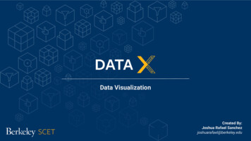
List of Figures1.1 Parallel coordinates display of Detroit Homicide data set: a 7-dimensionaldata set with 13 records. Note the inverse correlations between thenumber of cleared homicides and both the number of governmentworkers and the total number of homicides. . . . . . . . . . . . . . . .41.2 Parallel coordinates display of a Remote Sensing data set: a 5-dimensionaldata set with 16,384 records. Note the amount of over-plotting precludes the perception of any data trends, for instance the relativedensities. . . . . . . . . . . . . . . . . . . . . . . . . . . . . . . . . . .51.3 Various layouts in Pixel-Oriented Visualization. (a) using ScreenFilling Curve Techniques. (b) using Recursive Pattern Techniques.(c) Query-Dependent using Spiral and Snake- Spiral Techniques. (d)Query-Dependent using Snake-Axes and Grouping Techniques [Images generated in VisDB] . . . . . . . . . . . . . . . . . . . . . . . . .62.1 Wavelet approximations of a timeseries data set at different resolutions. [Image used from [WB96]] . . . . . . . . . . . . . . . . . . . . . 122.2 Using overplotting to reveal the internal structure of a data set. [Image used from [WL97]] . . . . . . . . . . . . . . . . . . . . . . . . . . 133.1 Flat Parallel Coordinates . . . . . . . . . . . . . . . . . . . . . . . . . 20v
3.2 Flat Star Glyphs . . . . . . . . . . . . . . . . . . . . . . . . . . . . . 203.3 Flat Scatterplot Matrices . . . . . . . . . . . . . . . . . . . . . . . . . 203.4 Flat Dimensional Stacking . . . . . . . . . . . . . . . . . . . . . . . . 203.5 Hierarchical Parallel Coordinates . . . . . . . . . . . . . . . . . . . . 253.6 Hierarchical Star Glyphs . . . . . . . . . . . . . . . . . . . . . . . . . 253.7 Hierarchical Scatterplot Matrices . . . . . . . . . . . . . . . . . . . . 253.8 Hierarchical Dimensional Stacking . . . . . . . . . . . . . . . . . . . . 254.1 HSI Color model used for the color mapping in pixel oriented displays. 354.2 Colormap Editor for pixel oriented displays in XmdvTool. . . . . . 374.3 Rectangular and Circular shapes of subwindows. . . . . . . . . . . . . 384.4 Rectangular and Circular segment arrangement of pixels. . . . . . . . 394.5 Subwindow placement by MDS algorithm for AAUP dataset. . . . . . 414.6 Brush region can be changed by moving the markers on the colormap. 434.7 Brush region can be changed through the auxiliary brush toolbox. . . 444.8 Data-space brushing is accomplished by Shift Mouse clicking andpainting over the subwindow. Note that the mouse cursor changes toa hand icon when brushing in data-space. . . . . . . . . . . . . . . . . 444.9 Distorted dimension for the AAUP dataset. . . . . . . . . . . . . . . 454.10 Manual Pixel Reordering sorted on Magnetics dimension on the Remote Sensing Dataset. . . . . . . . . . . . . . . . . . . . . . . . . . . 464.11 A comparison of the display of (a) full dataset and (b) sampleddataset of the remote sensing dataset. Both visualizations seem similar. 47vi
5.1 Structure-based brushing tool. (a) Hierarchical tree frame; (b) Contour corresponding to current level-of-detail; (c) Leaf contour approximates shape of hierarchical tree; (d) Structure-based brush; (e)Interactive brush handles; (f) Colormap legend for level-of-detail contour. . . . . . . . . . . . . . . . . . . . . . . . . . . . . . . . . . . 535.2 Structure-based brushing at two different levels-of-detail. . . . . . . . 555.3 A hierarchical parallel coordinates display of a remote sensing datasetwith the selected cluster painted in bold red to reflect that it is currently being brushed in the structure-based tool. The image on theright shows the corresponding level-of-detail indicated by the coloredcontour in the structure-based brush with the brushed region indicated by the wedge. In this case, we observe that the selected clustersshare the same mean value for magnetics and uranium contents, andhave high SPOT contents. . . . . . . . . . . . . . . . . . . . . . . . . 565.4 Hierarchical Pixel Oriented Display. . . . . . . . . . . . . . . . . . . . 585.5 Hierarchical Pixel Oriented Display at lod level of 0.2 for both brushedand unbrushed clusters for the UVW (6 dim - 150,000 data points) . 585.6 Hierarchical Pixel Oriented Display with brushed clusters at lod levelof 0.2 while unbrushed clusters at LOD level of 0.06. The dataset isthe UVW Dataset . . . . . . . . . . . . . . . . . . . . . . . . . . . . . 595.7 Hierarchical Pixel Oriented Display (Extents Visualization) with brushedclusters at LOD level of 0.2 while unbrushed clusters at LOD level of0.06. The dataset is the UVW Dataset . . . . . . . . . . . . . . . . . 605.8 Hierarchical Pixel Oriented Display (Extents Visualization) at LODlevel of 0.2 for both brushed and unbrushed clusters for the UVW (6dimensional - 150,000 data points)vii. . . . . . . . . . . . . . . . . . . 60
6.1 Class Diagram . . . . . . . . . . . . . . . . . . . . . . . . . . . . . . . 627.1 Linear functional dependency between dimensions 0 and 3 and quadraticfunctional dependency between dimensions 0 and 6. Note that thereis no dependency between dimension 0, 1 and 2 as they are completelydissimilar in appearance. . . . . . . . . . . . . . . . . . . . . . . . . . 697.2 Clustering can be easily seen in this view. Also note that the visualization tells us that the cluster is of a lower dimension than thedataset. . . . . . . . . . . . . . . . . . . . . . . . . . . . . . . . . . . 707.3 Pixel oriented visualization for the first data set and correspondingvisualization in Parallel Coordinates. Note that the pixel orienteddisplay shows the 4-D clusters. . . . . . . . . . . . . . . . . . . . . . . 727.4 Pixel oriented visualization for the fourth data set and correspondingvisualization in Parallel Coordinates. Note that the pixel orienteddisplay shows correspondence between dimensions 0, 3 and 6. . . . . . 73viii
List of Tables4.1 Parameters for generating color scales . . . . . . . . . . . . . . . . . . 367.1 Value ranges and dependencies for data items in the cluster of thirddata set. . . . . . . . . . . . . . . . . . . . . . . . . . . . . . . . . . . 72ix
Chapter 1IntroductionOur ability to generate and accumulate information has far exceeded our ability toeffectively process them. The ubiquitous exchange of information in this technologyage is a strong impetus for data growth. The proliferation of the internet todaycould only hint at the potential of tomorrow’s exponential information growth. Advancements in data acquisition technologies results in acquiring data at far greaterdensities and resolutions than ever before. Such evidence clearly puts forward a casethat data size is ever evolving and rising; and that in view of this growth it will beincreasingly difficult to process data in search of anomalies, patterns, features, andultimately knowledge and extrapolation of that knowledge.Interpreting data, be it overwhelming or not, is an arduous task. But it is mostdifficult when it is unclear what, in the voluminous data, to look out for. Automatedanalysis is hopeless when such analysis criteria cannot even be explicitly formulated.This is where visualization plays a crucial and most effective role — by relying uponthe power of the trained human eye.1
1.1Multivariate Data VisualizationMultivariate visualization simply refers to the display of multidimensional data. Amultidimensional data set consists of a collection of N -tuples, where each entryof an N -tuple is a nominal or ordinal value corresponding to an independent ordependent variable. We distinguish ourselves from the domain-specific class of visualization methods. Our research can be termed as non-domain-specific multivariatevisualization, a radically different mode of displaying multidimensional data. Itsnondomain specific nature results in generality and as such may be used to displaya much larger class of datasets. Examples of such datasets include results fromcensuses, surveys and simulations. Most analysis of such data to date still relieson the application of statistical computations. Statistical methods, though precise,lack the richness of graphical depictions. But more importantly, they require theuser to explicitly define sets of parameters for analysis. This is an arduous task, ifnot impossible, if the user has little knowledge or intuition about the characteristicsof the data that they are about to analyze.Visualization serves to complement rather than to replace traditional data analysis. Visualization is the graphical presentation of information, with the goal ofproviding the viewer with a qualitative understanding of the information contents.A visual sense of the data provides an interpretation unprecedented by statisticalmethods. It facilitates identification of trends and anomalies otherwise missed bystatistical analysis due to the difficulty of explicitly formulating analysis parameters.Observations from the visualization session may be further pursued using statistical methods supplied with parameters that befit the visual cues. These visual cueshelp the user to focus on where to target the quantitative or statistical analysis.Several techniques have been proposed to display non-domain-specific multivariate2
data. They have been broadly categorized [Kei00] as: Geometric Projection: These techniques aim to find interesting geometrictransformations and projections of multidimensional data sets. Examples include Scatterplot matrices [And72], Landscapes [Wri95], Hyperslice [WvL93]and Parallel Coordinates [ID90]. Icon-based : The idea here is to map each multidimensional data item to ashape, where data attributes control shape and color attributes. Examplesinclude Chernoff-faces [Che73], Stick figures [PG88], Shape Coding [Bed90],and Color Icons [Lev91]. Hierarchical : These techniques subdivide the k-dimensional space and presentthe subspaces in a hierarchical fashion. Examples include Dimensional Stacking [WLT96], Worlds-within-worlds [FB90], Treemap [Shn92], and Cone Trees[RMC91]. Pixel-based : Here, each attribute value is represented by one colored pixel andthe values for each attribute are presented in separate subwindows. Examples are spiral [KD94] [Kei96], recursive pattern [KKA95], and circle segmenttechniques [AKK96].The first three techniques do not scale well with respect to the size of the dataset. The main problem with applying such techniques to large data sets is displayclutter — that the amount of clutter obscures or occludes any visible trends inthe data display. For instance, take the parallel coordinates display in Fig. 1.1.We can easily spot correlations between variables in the data set. However, if wedisplay a larger data set as shown Fig. 1.2, we can hardly discern any relativepatterns or anomalies due to the mass of overlapping lines. As a generalization, we3
Figure 1.1: Parallel coordinates display of Detroit Homicide data set: a 7dimensional data set with 13 records. Note the inverse correlations between thenumber of cleared homicides and both the number of government workers and thetotal number of homicides.postulate that any method that displays a single entity per data point invariablyresults in overlapped elements and a convoluted display that is not suitable for thevisualization of large data sets. The quantification of the term “large” varies andis subject to revision in sync with the state of computing power. For our currentapplication, we define a large data set to contain tens of thousands to a million dataelements or more. Pixel-based displays are the only set of visualization techniquesthat aim to effectively visualize such large datasets.1.2Pixel Oriented VisualizationPixel-oriented techniques have been pioneered by Keim for the VisDB system [KD94]as a means for representing large amounts of high-dimensional data with respect to4
Figure 1.2: Parallel coordinates display of a Remote Sensing data set: a 5dimensional data set with 16,384 records. Note the amount of over-plotting precludes the perception of any data trends, for instance the relative densities.a given query. The basic idea of pixel-oriented visualization techniques is to represent each attribute value as a single colored pixel, mapping the range of possibleattribute values to a fixed color map and displaying different attributes in differentsubwindows. Pixel-oriented visualization techniques maximize the amount of information represented at one time without any overlap. They effectively preserve theperception of small regions of interest while still maintaining the global view.Designing pixel-oriented displays have been discussed at length in [Kei00]. Thedesign considerations are the choice of color space, subwindow shapes, pixel arrangement, dimension ordering and query specification. One of the most importantconsiderations in pixel-oriented displays is the arrangement of the pixels within eachof the subwindows. This is important since, due to the density of the pixel displays,only a good arrangement will lead to the discovery of clusters and correlations among5
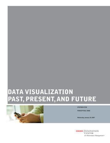
Figure 1.3: Various layouts in Pixel-Oriented Visualization. (a) using Screen-FillingCurve Techniques. (b) using Recursive Pattern Techniques. (c) Query-Dependentusing Spiral and Snake- Spiral Techniques. (d) Query-Dependent using Snake-Axesand Grouping Techniques [Images generated in VisDB]the dimensions. The arrangement defines the layout of the pixels within the display.Query-independent techniques use the natural ordering within the data (for example, time-series data) to define the layout, whereas Query-dependent techniquesarrange th
data visualization package, to incorporate pixel based techniques and to explore their strengths and weaknesses. The main challenge here was to seamlessly apply the interaction and distortion techniques used in other visualization methods within . 3.3