Transcription
STATISTICS REVIEWStatistics and the Scientific Method In general, the scientific method includes:1. A review of facts, theories, and proposals,2. Formulation of a logical hypothesis that can be evaluated by experimentalmethods, and3. Objective evaluation of the hypothesis on the basis of experimental results. Objective evaluation of a hypothesis is difficult because:1. It is not possible to observe all conceivable events (populations vs. samples) and2. Inherent variability exists because the exact laws of cause and effect are generallyunknown. Scientists must reason from particular cases to wider generalities.This is a process of uncertain inference.This process allows us to disprove hypotheses that are incorrect, but it does not allowus to prove hypotheses that are correct. Statistics is defined as the science, pure and applied, of creating, developing, andapplying techniques by which the uncertainty of inductive inferences may beevaluated. Statistics enables a researcher to draw meaningful conclusions from masses of data. Statistics is a tool applicable in scientific measurement. Its application lies in many aspects of the design of the experiment. This includes:1. Initial planning of the experiment,2. Collection of data,3. Analysis of results,4. Summarizing of the data, and5. Evaluation of the uncertainty of any statistical inference drawn from theresults.Types of variables1. Qualitative variable: One in which numerical measurement is not possible. An observation is made when an individual is assigned to one of severalmutually exclusive categories (i.e. cannot be assigned to more than onecategory). Non-numerical data. Observations can be neither meaningfully ordered nor measured (e.g. haircolor, resistance vs. susceptibility to a pathogen, etc.).
2. Quantitative variable:1. One in which observations can be measured.2. Observations have a natural order of ranking.3. Observations have a numerical value (e.g. yield, height, enzyme activity, etc.) Quantitative variables can be subdivided into two classes:1. Continuous: One in which all values in a range are possible (e.g. yield, height,weight, etc.).2. Discrete: One in which all values in a range are not possible, often counting data(number of insects, lesions, etc.).Steven’s Classification of Variables Stevens (1966)1 developed a commonly accepted method of classifying variables.1. Nominal variable: Each observation belongs to one of several distinct categories. The categories don’t have to be numerical. Examples are sex, hair color, race, etc.2. Ordinal variable: Observations can be placed into categories that can be ranked. An example would be rating for disease resistance using a 1-10 scale,where 1 very resistant and 10 very susceptible. The interval between each value in the scale is not certain.3. Interval variables: Differences between successive values are always the same. Examples would be temperature and date.4. Ratio variables: A type of interval variable where there is a natural zero point or originof measurement.1 Examples would be height and weight. The difference between two interval variables is a ratio variable.Stevens, S.S. 1966. Mathematics, measurement and psychophysics. pp. 1-49. In S.S. Stevens (ed.)Handbook of experimental psychology. Wiley, New York.
Descriptive measures depending on Steven’s scale†Classification Graphical measuresMeasures ofMeasures ofcentral tendencydispersionNominalBar graphsModeBinomial orPie chartsmultinomialvarianceOrdinalBar graphsHistogramMedianRangeIntervalHistogram areas aremeasurableMeanStandard deviationRatioHistogram areas are Geometric meanCoefficient ofmeasurableHarmonic meanvariation†Table adapted from Afifi, A., S. May, and V.A. Clark. 2012. Practical multivariateanalysis 5th edition. CRC Press, Taylor and Francis Group, Boca Raton, FL.Presenting variables1. Yi notation In this course, we are going to use the letter Y to signify a variable using theYi notation. Yi is the ith observation of the data set Y. (Y1, Y2, Y3 . . . Yn). If Y 1, 3, 5, 9, then Y1 and Y3 .2. Vector notation The modern approach to presenting data uses vectors. Y1Y2Y Y3.YnSpecifically, a vector is an ordered set of n elements enclosed by a pair ofbrackets.
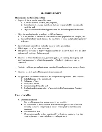
Using numbers from the previous example,1Y 359Y’ is called the transpose of Y.The transpose of a column vector is a row vector.Using the previous example, Y ' 1 3 5 9 Vector math A row and column vector can be multiplied if each vector has the same number ofelements. The product of vector multiplication is the sum of the cross products of thecorresponding entries. Multiplication between two column vectors requires taking the transpose of oneof the vectors. For example, if12X 3 and Y 4452X’Y 1 3 4 x 45X’Y (1*2) (3*4) (4*5) 34Probability Distributions The probability structure of the random variable y is described by its probabilitydistribution. If the variable y represents a discrete quantitative variable, we can call theprobability of the distribution of y, p(y), the probability function of y. If the variable y represents a continuous quantitative variable, we can call theprobability distribution of y, f(y), the probability density function of y. In the graph of a discrete probability function, the probability is represented bythe height of the function p(yi). In the graph of a continuous probability function, the probability is represented bythe area under the curve, f(y), for a specified interval.
p(y,)y1y2y3y4y5y6y7y8f(y,)Distribution of a discrete variableP(a y b)abDistribution of a continuous variabley9
Properties of Probability Distributionsy discrete:0 p(yj) 1P(y yj) p(yj) p(yj) 1all values of yjall values of yjy continuous: 0 f(y)P(a y b) baf ( y )dyf ( y )dy 1Populations vs. SamplesPopulation: Consists of all possible values of a variable. Are defined by the experimenter. Are characterized by parameters. Parameters usually are specified using Greek letters.Sample: Consists of part of the population. We often make inferences about populations using information gathered fromsamples. It is extremely important that samples be representative of the population. Samples are characterized by statistics.ItemMeanVarianceStandard deviationParameterStatisticµYs2sσσ2Three Measures of Central Tendency1. Mean (arithmetic)2. Median – Central value3. Mode – Most widely observed value
MeannY ( Yi ) / n ( Yi ) / ni 1 Where: Y mean,Yi is the ith observation of the variable Y, andn number of observations We can also use “Y dot” notation to indicate arithmetic functions. For example Fact: The sum of the deviations from the mean equals zero. Yi Y. where the “.” means summed across all i. (Y Y ) 0iExample of Calculating the MeanYi951412 Yi Yi Y9-10 -15-10 -514-10 412-10 240 (Y Y ) 0Step 1. Calculatei Yi (9 5 14 12) 40Step 2. Divide Yi by n(40/4) 10 Use of the mean to calculate the sum of squares (SS) allows the calculation of theminimum sum of square.SS (Yi Y ) 2 The mathematical technique that we will be using in this course for most of ourstatistical analyses is called the Least Squares Method.
Weighted Mean An arithmetic technique used to calculate the average of a group of means that do nothave the same number of observations. Weighted mean Yw niYi / niExample of Calculating a Weighted MeanMean grain protein of barley grown in three North Dakota Counties.CountyniYiCassTraillGrand Forks57313.5%13.0%13.9%Yw [5(13.5) 7(13.0) 3(13.9)] /(5 7 3) 13.34% Non-weighted mean would be (13.5 13.0 13.9)/3 13.47%Median Value for which 50% of the observations, when arranged in order from low to high,lie on each side. For data with a more or less normal distribution, the mean and median are similar. For skewed data, data with a pronounced tail to the right or left, the median often is a“better” measure of central tendency. The median often is used as the measure of central tendency when discussing dataassociated with income.Example of Determining the MedianLet Y 14, 7, 4, 17, 19, 10, 11Step 1. Arrange the data from low to high4, 7, 10, 11, 14, 17, 19Step 2. Identify the middle observation. This value is the median11 If the number of observations in a data set is an even number, the median is equal tothe average of the two middle observations.
Mode Value that appears most often in a set of data. There can be more than one value for the mode.Three Measures of Dispersion1. Variance2. Standard deviation3. Range Measures of dispersion provide information on the variability present in the data set. For example, given you have two data sets with the same mean:Y1 1, 3, 5, 7 Y 1 4Y2 1, 2, 3, 10 Y 2 4 By looking at only the means, we cannot determine anything about the variabilitypresent in the data. However, by determining the variance, standard deviation, or range for each data set,we can learn more about the variability present.Range The range is the difference between the maximum and minimum value in the data set. For example the range for Y1 7-1 6 and the range for Y2 10-1.Variance of a SampleDefinition formula: s 2 2Working formula:(Yi Y ) 22s Yi (n 1)( Y i) 2n(n 1) The numerator of the formula is called the sum of squares (SS). The denominator of the formula is called the degrees of freedom (df).
df number of observations – number of independent parameters being estimated o A data set contains n observations, the observations can be used either toestimate parameters or variability.o Each item to be estimated uses one df.o In calculating the sample variance, one estimate of a parameter is used, 𝒀.o This leaves n-1 degrees of freedom for estimating the sample variance.The parameter being estimated by 𝑌 is the population mean µ. Example of Calculating the Variance Using the Definition FormulaUsing the previous data of:s2(Y Y ) iY1 1, 3, 5, 7 and Y 1 4Y2 1, 2, 3, 10 and Y 2 42(n 1)2222s12 [(1 4) (3 4) (5 4) (7 4) ](4 1)2222s22 [(1 4) (2 4) (3 4) (10 4) ] 6.67(n 1) 16.67It would be very difficult and time consuming to calculate the variance using thedefinition formula; thus, the working formula generally is used to calculate thevariance.Example of Calculating the Variance Using the Working Formula2s 2 Yi ( Y i) 2n(n 1)2s12 (12 32 5 2 7 2 ) (1 3 45 7 ) (n 1)84 6.6725643
Variance of a Population The variance of a population has a slightly different formula than the variance of asample.σ 2 (Yi µ ) 2 NWhere Yi the ith observation in the population,µ Population mean, andN number of observations in the population. The denominator is different in that we do not calculate the df. Calculation of the df is not needed since there is no parameter being estimated.Standard Deviation Equal to the square root of the variance.s s2σ σ2Variance of the Mean and the Standard Deviation of the MeanGiven the following means, each with a different numbers of individuals:CountyniCassTraillGrand Forks573Yi13.5%13.0%13.9%First look at the thoughts of the variance of the mean In the table above, which mean do you think is the best? Why? Would you expect the variability of the mean based on 7 seven observations to beless than one based on 5 or 3 observations? In fact, we should not be surprised to learn that sample means are less variablethan single observations because means tend to cluster closer about some centralvalue than do single observations.
A different approach to looking at the variance of the mean From a population containing N observations, we can collect any number ofrandom samples of size n. We can plot the distribution of these n means. The distribution of all these n means is called “The distribution of the samplemean.” The distribution of the sample mean, like any other distribution, has a mean, avariance, and a standard deviation.There is a known relationship between the variance among individuals and thatamong means of individuals. This relation and the one for the standard deviation are:σ Y2 Thus:sY2 σ2nAndσY n σn22snσ2AndsY ss nn The standard deviation of the mean is more commonly referred to as theStandard Error.Coefficient of Variation (CV) The CV is a relative measure of the variability present in your data. To know if the CV for your data is large or small takes experience with similar data. The size of the CV is related to the experimental material used. Data collected using physical measurements (e.g. height, yield, enzyme activity, etc.)generally have a lower CV than data collected using a subjective scale (e.g. lodging,herbicide injury, etc.)%CV ( s ) *100YExample of use of the CV for checking data for problems Typically, a single CV value is calculated for the experiment; however, a CV can alsobe calculated for each treatment.
If the experiment CV is larger than expected, one can look at the CV values for eachtreatment to see if one or more of them are causal of the experiment CV. The individual treatment CVs can be calculated using a program such as E2E3Expt meanExpt. Standard deviationExpt. 3.580.379.269.075.381.017.6Treatment CV11.023.649.73.36.921.8Linear Additive Model We try to explain things we observe in science using models. In statistics, each observation is comprised of at least two components:1. Mean ( µ )2. Random error ( ε i ).Thus, the linear model for any observation can be written as:Yi µ εi
Mean, Variance, and Expected Values The mean, µ, of a probability distribution is a measure of its central tendency.Mathematically, the mean can be defined as: all y yp(y) y discrete µ y continuous f ( y )dy The mean also can be expressed as the expected value, where µ E(y). all y yp(y) y discrete µ E(y) y continuous f ( y )dy The variability or dispersion of a probability distribution can be measured by thevariance, defined as: ( y µ )2 p(y) all yσ2 2 ( y µ ) f ( y )dy y discretey continuousThe variance also can be expressed as an expectation as:σ2 E[(y-µ)2] V(y)Summary of Concepts of Expectation1. E(c) c2. E(y) µ3. E(cy) cE(y) cµ4. V(c) 05. V(y) σ26. V(cy) c2V(y) c2σ2If there are two random variables y1, with E(y1) µ1 and V(y1) σ 12 , and y2, withE(y2) µ2 and V(y2) σ 22 , then
7. E(y1 y2) E(y1) E(y2) µ1 µ28. V(y1 y2) V(y1) V(y2) 2Cov(y1, y2)Where Cov(y1, y2) E[(y1 - µ1)(y2-µ2)] and this is the covariance of the randomvariables y1 and y2. If y1 and y2 are independent, the Cov(y1, y2) 0.9. V(y1-y2) V(y1) V(y2) – 2Cov(y1, y2)If y1 and y2 are independent, then:10. V(y1 y2) V(y1) V(y2) σ 12 σ 22 .11. E(y1 . y2) E(y1) . E(y2) µ1 . µ2.However, note that12. y E ( y1 )E 1 y2 E ( y2 )Mean and Variance of a Linear Function Given a single random variable, y1, and the constant a1:Then E(a1y1) a1E(y1) a1µ1andV(a1y1) a12V ( y1 ) a12σ 12 Given the y1 and y2 are random variables and a1 and a2 are constants:Then E(a1y1 a2y2) a1E(y1) a2E(y2) a1µ1 a2µ2andV(a1y1 a2y2) a12V ( y1 ) a22V ( y2 ) 2a1a2Cov ( y1 , y2 ) a12σ 12 a22σ 22 2a1a2Cov ( y1 , y2 ) If there is no correlation between y1 and y2, thenV(a1y1 a2y2) a12V ( y1 ) a22V ( y2 )
Expectation of the Sample Mean and the Sample VarianceSample mean n yi 1 n1 nE ( y ) E i 1 E ( yi ) µ µ n n i 1n i 1 This relationship works because each yi is an unbiased estimator of µ.Sample variance n2 ( yi y ) n 11 E ( S 2 ) E E i 1E ( yi y ) 2 E ( SS )n 1 n 1 i 1 n 1 where
n E ( SS ) E ( yi y ) 2 i 1 nnn E yi i 1 2 y yi i 1 y 2 i 1 n nn E yi i 1 2 y 2 i 1 y 2 i 1 nn E yi i 1 y 2 i 1 σ 2 because σ 2 E(yi2 ) µ 2 and E ( y 2 ) µ 2 n n E yi2 ny 2 i 1 we getn ( µ 2 σ 2 ) n( µ 2 σ2i 1n) n( µ 2 σ 2 ) nµ 2 σ 2 nµ 2 nσ 2 nµ 2 σ 2 nσ 2 σ 2 (n 1)σ 2Therefore,1E (S 2 ) E ( SS ) σ 2n 1Thus, we can see that S2 is an unbiased estimator of σ2.Central Limit TheoremDefinition: The distribution of an average tends to be Normal, even if the distributionfrom which the average is computed is non-Normal.
SAS COMMANDS FOR UNIVARIATE ANALYSISoptions pageno 1;data example;input y1 y2;datalines;3 84 1011 85 135 812 128 137 10;;ods rtf file 'example.rtf';proc print;*comment this procedure statement will print the data.;title 'Output of Proc Print Statement';*comment a title statement following the procedure (proc) statementwill give a title for the output related to the proc statement. thetitle must be within single quotes.;proc means mean var std min max range stderr cv;*comment mean mean var variance std standard deviation min minimumvalue max maximum value range range stderr standard error cv coefficient ofvariation.;var y1 y2;title 'Output of Proc Means Statement';run;ods rtf close;Run;
Output of Proc Print StatementObs y1 y21324 103118845 13558612 1278 1387 10
Output of Proc Means StatementVariabley1y2MeanVarianceStd DevMinimumMaximumRangeStdCoeff ofError .00012.00013.0009.0005.0001.1560.77347.57521.342
1 Stevens, S.S. 1966. Mathematics, measurement and psychophysics. pp. 1-49. In S.S. Stevens (ed.) Handbook of experimental psychology. Wiley, New York. Descriptive measures depending on Steven’s scale† Classific