Transcription
STAT COE-Report-29-2017Understanding Analysis ofVarianceBest PracticeAuthored by: Cory Natoli21 December 2017The goal of the STAT COE is to assist in developing rigorous, defensible teststrategies to more effectively quantify and characterize system performanceand provide information that reduces risk. This and other COE products areavailable at www.afit.edu/STAT.STAT Center of Excellence2950 Hobson Way – Wright-Patterson AFB, OH 45433
STAT COE-Report-29-2017ContentsExecutive Summary . 2Introduction . 2Method . 3One-Way ANOVA . 3Motivating example . 3Model . 3Model Building . 3Assumptions . 4Hypotheses . 4Test Statistic . 6Decision . 7Multifactor ANOVA . 8Motivating example . 8Model . 8Hypotheses . 9Decision . 9Example . 10R Code. 11JMP . 14Conclusion . 16References . 17
STAT COE-Report-29-2017Executive SummaryAn important step in the DOE process is determining which factors truly affect the (numeric)response variable. A solution to this problem is through the use of analysis of variance (ANOVA). ANOVAis a procedure that uses hypothesis testing to determine whether the factor effects of two or morefactors are the same. This paper seeks to explain the basic statistical theory behind one-way ANOVA, aswell as detail the process and how to utilize ANOVA conceptually. Code is provided to perform ANOVA inR and JMP.Keywords: ANOVA, DOE, statistically significant, hypothesis testing, R, JMPIntroductionAnalysis of Variance (ANOVA) is a common technique for analyzing the statistical significance ofa number of factors in a model. The overall goal of ANOVA is to select a model that only contains termsthat add valuable insight in determining the value of the response, or in other words, a model that onlyincludes statistically significant terms. Assuming the data comes from a designed experiment, theanalysis will answer the question “Does this (do these) factor(s) cause a statistically significant differencein the response variable?” An important step in the design of experiments (DOE) process is determiningwhich variables truly affect the response, and ANOVA allows us to do this when the response iscontinuous. In order to understand the concepts of ANOVA, this paper begins with an introduction toANOVA when there is only one factor (one-way ANOVA), and then connects the concepts to multifactorANOVA. ANOVA can only be used if the response variable is quantitative; it will not work for qualitativeresponses. All factors in the model are treated as if they are qualitative (categorical) variables. Theresults tell us whether or not there is a difference in the average response at the various levels of thefactor. If the data do not fulfill these requirements (i.e. the response is qualitative, the goal is prediction,etc.), it is possible that regression is better suited for the analysis as it is a more general method.Before diving into the concepts, we first establish the notation associated with ANOVA. 𝑥𝑥̅ is the mean of a sample of data, 𝑥𝑥1 , 𝑥𝑥2 , , 𝑥𝑥𝑛𝑛 ; the bar simply denotes “arithmeticaverage.”𝑥𝑥 is the estimated value for x; the hat denotes that it is a predicted value from data.𝑥𝑥. is the value of the x values summed over all levels of the factor in which the “.” replaces.Formulas are provided for all of the values discussed to further increase conceptualunderstanding, but the values can be calculated using statistical software (examples shown indetail later).Page 2
STAT COE-Report-29-2017MethodOne-Way ANOVAMotivating exampleWe use a simple example to demonstrate the one-way ANOVA scenario. Suppose there is a newmissile being tested and we wish to characterize the miss distance. In this scenario, the miss distance isthe response variable. We determine there is only one factor, distance to the target, that affects themiss distance. Therefore, we wish to determine if this solitary factor has a statistically significant effecton the miss distance.Table 1. Generic data table for one factor experimentFactor LevelObservations1𝑦𝑦11 𝑦𝑦12 𝑦𝑦1𝑛𝑛2 𝑣𝑣𝑦𝑦21 𝑦𝑦𝑣𝑣1𝑦𝑦22 𝑦𝑦𝑣𝑣2 𝑦𝑦2𝑛𝑛 ��𝑦 1.𝑦𝑦𝑣𝑣.𝑦𝑦 𝑣𝑣.𝑦𝑦2. 𝑦𝑦.𝑦𝑦 2. 𝑦𝑦 .ModelIn order to conduct ANOVA, one must first establish the mathematical model. The model for one-wayANOVA is as follows: 𝑌𝑌𝑖𝑖𝑖𝑖 𝜇𝜇 𝜏𝜏𝑖𝑖 𝜖𝜖𝑖𝑖𝑖𝑖 where 1 𝑡𝑡 𝑟𝑟𝑖𝑖 , 1 𝑖𝑖 𝑣𝑣 , 𝜖𝜖 𝑖𝑖𝑖𝑖𝑖𝑖 𝑁𝑁(0, 𝜎𝜎 2 )𝑌𝑌𝑖𝑖𝑖𝑖 is the 𝑡𝑡th observation at the 𝑖𝑖 th level of the factor𝑟𝑟𝑖𝑖 is the number of observations in factor level i𝜇𝜇 is the overall mean of the response𝜏𝜏𝑖𝑖 is the effect of the ith factor level on the response𝜖𝜖𝑖𝑖𝑖𝑖 is the random error, assumed to be independently and identically normally distributedwith mean 0 and constant variance 𝜎𝜎 2 (𝑖𝑖𝑖𝑖𝑖𝑖 𝑁𝑁(0, 𝜎𝜎 2 ))𝑣𝑣 is the number of factor levels being testedThe factor effect 𝜏𝜏𝑖𝑖 measures the change in the response due to the 𝑖𝑖 th factor level. These factoreffects are parameters in the model that must be estimated using the test data.Model BuildingThe model includes a single term for the factor for which we wish to determine the significancethrough the use of ANOVA. Since there is just one factor of interest, this is the simplest case of ANOVA.If the term is significant, we leave the model as written above and it can be used as the empirical modelfor the system. However, if the term is determined not to be significant, we can reduce the model toPage 3
STAT COE-Report-29-2017𝑌𝑌𝑖𝑖𝑖𝑖 𝜇𝜇 𝜖𝜖𝑖𝑖𝑖𝑖In other words, the model to predict the response no longer includes a factor effect – the response issimply the mean plus some random error. This paper begins by introducing the concepts that allow adecision to be made on the significance of a single factor and then extends the process to the morerealistic scenario where a system is characterized by many factors.AssumptionsANOVA requires a set of assumptions to be met or the results will not be valid. The assumptions are: Error terms are independent, normally distributed with mean 0 and variance 𝜎𝜎 2All levels of each factor follow a normal distributionVariance, 𝜎𝜎 2 , is the same across all levels of each factorObservations are independentThese are the same assumptions that are necessary for building a regression model. Moreinformation on these can be found in “The Model Building Process Part 1: Checking model Assumptions”best practice (Burke 2017).HypothesesIf the factor in the experiment has 𝜈𝜈 levels, we can use ANOVA to test for equality of factoreffects. The null hypothesis states that the factor has no effect on the response as indicated by the factthat all factor terms in the model vanish:𝐻𝐻0 : {𝜏𝜏1 𝜏𝜏2 𝜏𝜏𝑣𝑣 0}The alternative hypothesis states that the factor has an effect on the response because at least onefactor term in the model is non-zero:𝐻𝐻𝑎𝑎 : {𝑁𝑁𝑁𝑁𝑁𝑁 𝑎𝑎𝑎𝑎𝑎𝑎 𝜏𝜏𝑖𝑖 𝑒𝑒𝑒𝑒𝑒𝑒𝑒𝑒𝑒𝑒 0}The concept of ANOVA revolves around comparing the “within” factor variance with the“between” factor mean variances. This comparison is done by partitioning the total variability of theresponse into two important components: sum of squares for error (SSE) and sum of squares for factors(SSR). SSR measures the difference between factor level means; SSE, the difference within a factor levelto the factor level mean can only be due to random error (Montgomery, 2017).The total sum of squares (SST) measures the total variability in the response and is defined as𝑣𝑣𝑟𝑟𝑖𝑖𝑆𝑆𝑆𝑆𝑆𝑆 (𝑦𝑦𝑖𝑖𝑖𝑖 𝑦𝑦 . )2𝑖𝑖 1 𝑡𝑡 1Page 4
STAT COE-Report-29-2017SST can be decomposed into SSE and SSR. SSE, the “within” factor variance, is calculated as𝑟𝑟𝑖𝑖𝑣𝑣where 𝑦𝑦 𝑖𝑖. 𝑟𝑟𝑖𝑖 𝑦𝑦 𝑡𝑡 ���𝑆 (𝑦𝑦𝑖𝑖𝑖𝑖 𝑦𝑦 𝑖𝑖 . )2𝑖𝑖 1 𝑡𝑡 1. SSE is also called the error sum of squares.SSR, the “between” factor variance, is the value “used in describing how well a model represents the data being modeled” (Explained sum of squares 2017). SSR is calculated as𝑣𝑣where 𝑦𝑦 . 𝑟𝑟𝑖𝑖 𝑦𝑦 𝑣𝑣𝑖𝑖 1 𝑡𝑡 1𝑖𝑖𝑖𝑖𝑛𝑛𝑆𝑆𝑆𝑆𝑆𝑆 𝑟𝑟𝑖𝑖 (𝑦𝑦 𝑖𝑖. 𝑦𝑦 . )2𝑦𝑦𝑖𝑖 1 . . SSR is the variability between the means of each factor level.𝑛𝑛Figure 1 shows a visual decomposition of these sums of squares. In the figure, the blue linerepresents the predicted values for a given model. The black dots are the actual data points. SSE iscalculated from the difference between the actual point and the predicted value, SSR is calculated fromthe difference between the predicted value and the grand mean, and sum of squares total, SST, is thesum of SSE and SSR. The estimated values for 𝜇𝜇 and 𝜏𝜏 are the values that minimize the SSE.SSESSTSSR𝑦𝑦 Figure 1: Decomposing Sum of SquaresPage 5
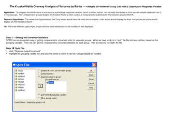
STAT COE-Report-29-2017Test StatisticSSE and SSR are used to conduct the hypothesis test on the factor effects. The ANOVAframework uses an F-statistic to compare the means of the different factor levels. The idea behind the Fstatistic is to compare the ratio of the between factor variability vs the within factor variability (𝐹𝐹 ���𝑏" 𝑓𝑓𝑓𝑓𝑓𝑓𝑓𝑓𝑓𝑓𝑓𝑓 ��𝑣𝑣𝑣"within" factor variance) in order to make a decision on a difference in means.Figure 2 shows the difference between the “between” and “within” variances, as well as anumber of different scenarios for large and small “between” factor variance and “within” factorvariance. The “between” variance is the variance between the three different curves. The “within”variance is the variance within a single curve. Essentially, if the “between” variance is much larger thanthe “within” variance, the factor is considered statistically significant. Recall, ANOVA seeks to determinea difference in means at each level of a factor. If the factor level impacts the mean, then that factor isstatistically significant. The image in the top right shows the most obvious case of this instance. Whenthe difference in the means is large, this implies the “between” group variation is large. The variancewithin groups is also small, so we can clearly identify the effect on the response caused by that factor.Conversely, the bottom left demonstrates a scenario with a larger “within” factor variance and a small“between” factor variance, as the means are close together and there is a lot of overlap in thedistributions. This may be a scenario in which the factor is not statistically significant.Figure 2: Conceptual ANOVAPage 6
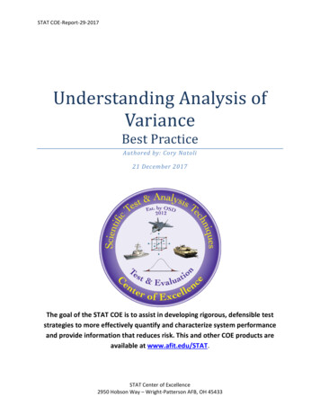
STAT COE-Report-29-2017Decisions are hardest to make when there is large variance within factors or the means betweenthe factor levels are close. If there is a large variance within factors, there is a lot of overlap between thedistributions and it makes determining significance much more difficult. Also if the means are close, itwould follow that stating the means are different is difficult.DecisionA large value for the F statistic suggests evidence against the null hypothesis. The naturaldecision is to then reject the null hypothesis. Conversely, a small value for the F statistic suggests thedata support the null hypothesis and the decision is to fail to reject the null �𝑅𝑅 𝐻𝐻0 𝑖𝑖𝑖𝑖𝑆𝑆𝑆𝑆𝑆𝑆/(𝑣𝑣 1) 𝐹𝐹𝛼𝛼,𝑣𝑣 1,𝑛𝑛 𝑣𝑣𝑆𝑆𝑆𝑆𝑆𝑆/(𝑛𝑛 𝑣𝑣)Where 𝐹𝐹𝛼𝛼,𝑣𝑣 1,𝑛𝑛 𝑣𝑣 represents a cut-off value at 𝛼𝛼-level of significance. We can also make a decisionbased on the p-value. Figure 3 shows how a p-value is calculated for an F-distribution. The p-value is theprobability of observing the test statistic or something more extreme given the null hypothesis is true.The probability shaded in the figure represents the p-value. A p-value smaller than the significance level(𝛼𝛼 level, set prior to the experiment, often 0.1 or 0.05) provides evidence against the null hypothesisand leads to concluding the alternative hypothesis is true (at least one factor effect is nonzero). If the pvalue is larger than 𝛼𝛼, the decision is to fail to reject the null hypothesis.Figure 3. F distributionMost commonly, calculations associated with ANOVA are presented in an ANOVA table. Table 2 shows ageneric ANOVA table.Page 7
STAT COE-Report-29-2017Table 2. Generic ANOVA TableSourceDegrees ofSum ofMean SquareF-RatioP-ValueFreedomSquares𝑣𝑣 1FactorsSSRMSR SSR/𝑣𝑣 1MSR/MSECalculated𝑛𝑛 𝑣𝑣ErrorSSEMSE SSE/ 𝑛𝑛 𝑣𝑣𝑛𝑛 1TotalSST 𝑛𝑛 is the total sample size and is equal to 𝑣𝑣𝑖𝑖 1 𝑟𝑟𝑖𝑖 P-value is calculated by software (see on.aspxfor technical details)Multifactor ANOVAMotivating exampleContinuing with the missile example, suppose we determine there are two factors that mayaffect the miss distance. Now, instead of simply looking at distance from the target, we are alsointerested in the height of the launch. Our model must be modified to reflect this change.ModelOnce again, the model is the foundation of all calculations. Terms are added to the one-factormodel to accommodate the main effects of additional factors, and more terms may be added to includeinteractions between factors. After adding the main effect term for the new factor and a term for factorinteraction, our new two-factor model is𝑌𝑌𝑖𝑖𝑖𝑖𝑖𝑖 𝜇𝜇 𝛼𝛼𝑖𝑖 𝛽𝛽𝑗𝑗 (𝛼𝛼𝛼𝛼)𝑖𝑖𝑖𝑖 𝜖𝜖𝑖𝑖𝑖𝑖𝑖𝑖 𝑤𝑤ℎ𝑒𝑒𝑒𝑒𝑒𝑒 1 𝑡𝑡 𝑟𝑟𝑖𝑖 , 1 𝑖𝑖 𝑎𝑎 , 1 𝑗𝑗 𝑏𝑏 , 𝜖𝜖 𝑖𝑖𝑖𝑖𝑖𝑖 𝑁𝑁(0, 𝜎𝜎 2 ) 𝑌𝑌𝑖𝑖𝑖𝑖𝑖𝑖 is the tth observation at the ith factor A level and jth factor B level.𝜇𝜇 is the overall mean𝛼𝛼𝑖𝑖 is the factor effect of factor A at level I; 𝑎𝑎𝑖𝑖 1 𝛼𝛼𝑖𝑖 0𝛽𝛽𝑗𝑗 is the factor effect of factor B at level j; 𝑏𝑏𝑗𝑗 1 𝛽𝛽𝑗𝑗 0(𝛼𝛼𝛼𝛼)𝑖𝑖𝑖𝑖 represents the interaction effect of factors A and B; 𝑖𝑖(𝛼𝛼𝛼𝛼)𝑖𝑖𝑖𝑖 0 , 𝑗𝑗 1, , 𝑏𝑏; 𝑗𝑗(𝛼𝛼𝛼𝛼)𝑖𝑖𝑖𝑖 , 𝑖𝑖 1, , 𝑎𝑎𝜖𝜖𝑖𝑖𝑖𝑖𝑖𝑖 is the random errorThis model can be extended to three or more factors by including the additional corresponding terms.𝑌𝑌𝑖𝑖𝑖𝑖𝑖𝑖 𝑡𝑡 𝜇𝜇Overall mean 𝛼𝛼𝑖𝑖 𝛽𝛽𝑗𝑗 𝛾𝛾𝑘𝑘 These factors make up the main effects model (𝛼𝛼𝛼𝛼𝛼𝛼)𝑖𝑖𝑖𝑖𝑖𝑖 3-factor interactions (𝛼𝛼𝛼𝛼)𝑖𝑖𝑖𝑖 (𝛼𝛼𝛼𝛼)𝑖𝑖𝑖𝑖 (𝛽𝛽𝛽𝛽)𝑗𝑗𝑗𝑗 2-factor interactionsPage 8
STAT COE-Report-29-2017 Higher-order interactions (dependent on number of factors) 𝜖𝜖𝑖𝑖𝑖𝑖𝑖𝑖 𝑤𝑤ℎ𝑒𝑒𝑒𝑒𝑒𝑒 1 𝑡𝑡 𝑟𝑟𝑖𝑖 , 1 𝑖𝑖 𝑎𝑎 , 1 𝑗𝑗 𝑏𝑏, 1 𝑘𝑘 𝑐𝑐 , 𝜖𝜖 𝑖𝑖𝑖𝑖𝑖𝑖 𝑁𝑁(0, 𝜎𝜎 2 )Similar to the one-way ANOVA scenario, the model includes terms for the factors, or factors thatwe wish to determine significance for through the use of ANOVA. In this situation, we are able toperform a hypothesis test on each term, both for main effects and interactions, to determinesignificance. In order to maintain model hierarchy, we never want to remove a lower order term that issignificant in a higher order interaction term. For example, we would not remove 𝛼𝛼𝑖𝑖 if the modelcontained (𝛼𝛼𝛼𝛼), the interaction between A and B. The idea is to build the best fitting, and easiest tointerpret, model possible. We test each term and reduce the model as necessary until this goal isachieved.For conceptual understanding, this paper focuses on the two-factor model.HypothesesThe hypotheses for multifactor ANOVA have the same simple interpretation, but are done for allthe main effects and interaction effects. The hypotheses for the main effect terms are as follows:For factor A 𝐻𝐻0 : 𝐹𝐹𝐹𝐹𝐹𝐹𝐹𝐹𝐹𝐹𝐹𝐹 𝐴𝐴 ℎ𝑎𝑎𝑎𝑎 𝑁𝑁𝑁𝑁 𝑒𝑒𝑒𝑒𝑒𝑒𝑒𝑒𝑒𝑒𝑒𝑒 𝑜𝑜𝑜𝑜 𝑡𝑡ℎ𝑒𝑒 ��𝑟𝑟𝑟For factor B 𝐻𝐻0 : 𝐹𝐹𝐹𝐹𝐹𝐹𝐹𝐹𝐹𝐹𝐹𝐹 𝐵𝐵 ℎ𝑎𝑎𝑎𝑎 𝑁𝑁𝑁𝑁 𝑒𝑒𝑒𝑒𝑒𝑒𝑒𝑒𝑒𝑒𝑒𝑒 𝑜𝑜𝑜𝑜 𝑡𝑡ℎ𝑒𝑒 ��𝑟𝑟𝑟Both share the same alternative hypothesis of 𝐻𝐻𝑎𝑎 : 𝑇𝑇ℎ𝑒𝑒 𝑓𝑓𝑓𝑓𝑓𝑓𝑓𝑓𝑓𝑓𝑓𝑓 𝐻𝐻𝐻𝐻𝐻𝐻 𝑎𝑎𝑎𝑎 𝑒𝑒𝑒𝑒𝑒𝑒𝑒𝑒𝑒𝑒𝑒𝑒 𝑜𝑜𝑜𝑜 𝑡𝑡ℎ𝑒𝑒 ��𝑟𝑟𝑟.The hypothesis for an interaction term is as follows:𝐻𝐻0 : The interaction effect AB has NO effect on the responseDecision𝐻𝐻𝑎𝑎 : The interaction effect AB HAS an effect on the response0nce again, there is a decision rule based off the F-distribution that isReject H0 𝑓𝑓𝑓𝑓𝑓𝑓 ���𝑓𝑓𝑓 ��𝑓𝑓𝑓𝑓𝑓 ,𝑑𝑑𝑓𝑓𝐸𝐸 𝐹𝐹(𝑎𝑎 1)(𝑏𝑏 1)(𝑟𝑟 �/𝑑𝑑𝑓𝑓𝐸𝐸Where 𝑑𝑑𝑑𝑑 is the degrees of freedom. Degrees of freedom are the number of independent elements inthat sum of squares (Montgomery, 2017). As before, the F-ratios will be converted into p-values to assistthe decision. Once again, we will use software to calculate the ANOVA table. The two-factor ANOVAtable is shown in Table 3.Page 9
STAT COE-Report-29-2017Table 3. ANOVA table for a two-factor studySourceFactor AFactor BABErrorTotal Degrees ofFreedom𝑎𝑎 1𝑏𝑏 1(𝑎𝑎 1)(𝑏𝑏 1)𝑛𝑛 𝑎𝑎𝑎𝑎𝑛𝑛 1Sum ofSquaresSSASSBSSABSSESSTMean SquareF-RatioP-Value𝑀𝑀𝑀𝑀𝑀𝑀 𝑆𝑆𝑆𝑆𝑆𝑆/(𝑎𝑎 1)𝑀𝑀𝑀𝑀𝑀𝑀 𝑆𝑆𝑆𝑆𝑆𝑆/(𝑏𝑏 1)MSAB SSAB/(𝑎𝑎 1)(𝑏𝑏 1)MSE SSE/(𝑛𝑛 alculatedCalculatedP-value will be calculated by software or see on.aspx fortechnical detailsAfter the ANOVA process, the model can be simplified by removing terms that are not statisticallysignificant. However, a lower order term cannot be removed from the model if it is included in a higherorder term that will be retained. For example, if Factor B has a large p-value which indicates it is notsignificant, but AB has a very small p-value that indicates it is significant, then Factor B cannot beremoved from the model.ExampleConsider a sensor assessment study with two factors, slant range and look down angle, whichmay impact the target location error (TLE). This is an example of a two-factor ANOVA.Figure 4: summary of data for a TLE test with two factors, slant range and look down angleThe dataset has 12 observations consisting of 4 observations at different combinations of lookdown angle and slant range with 2 additional replicates. The model we wish to analyze is:𝑌𝑌𝑖𝑖𝑖𝑖𝑖𝑖 𝜇𝜇 𝛼𝛼𝑖𝑖 𝛽𝛽𝑗𝑗 (𝛼𝛼𝛼𝛼)𝑖𝑖𝑖𝑖 𝜖𝜖𝑖𝑖𝑖𝑖𝑖𝑖 𝑤𝑤ℎ𝑒𝑒𝑒𝑒𝑒𝑒 1 𝑡𝑡 3, 1 𝑖𝑖 2 , 1 𝑗𝑗 2 , 𝜖𝜖 𝑖𝑖𝑖𝑖𝑖𝑖 𝑁𝑁(0, 𝜎𝜎 2 )Page10
STAT COE-Report-29-2017 𝜇𝜇 is the overall mean𝛼𝛼𝑖𝑖 is the factor effect of slant range at level i𝛽𝛽𝑗𝑗 is the factor effect of look down angle at level j (𝛼𝛼𝛼𝛼) is the interaction of slant range and look down angle 𝜖𝜖𝑖𝑖𝑖𝑖 is the random errorWe will use both R and JMP to analyze the data at an alpha 0.05 level.R Code Load the Data. This example loads a comma separated values file with the data.TLE.example - read.csv(" /Documents/TLE example.csv") Check that the data has loaded properlyTLE.example########################## 123456789101112Angle Range TLE1-1 221-1 251-1 1911511 1511 10-11 56-11 51-11 61-1-1 35-1-1 37-1-1 36Attach the dataset to the variables, otherwise all variables must haveTLE.example VariableName. This step is optional but helps keep the code cleaner and savestime.attach(TLE.example) Fit the model. This can also be coded as TLEfit -aov(TLE Angle Range Angle:Range,data TLE.example)TLEfit - aov(TLE Angle*Range, data TLE.example) Check the assumptionsplot(TLEfit)Page11
STAT COE-Report-29-2017 Create the ANOVA tableanova(TLEfit)####################Analysis of Variance TableResponse: TLEDf Sum Sq Mean Sq F valuePr( F)Angle127002700180.0 9.123e-07 ***Range148483.20.1114Angle:Range 176876851.2 9.658e-05 ***Residuals812015--Signif. codes: 0 '***' 0.001 '**' 0.01 '*' 0.05 '.' 0.1 ' ' 1Page12
STAT COE-Report-29-2017We can note the p-values [Pr( F) in R] to determine which factors are significant in the model. BothAngle and Angle*Range, the two-factor interaction, are significant with small P-values, while Range isnot significant. However, Range should not be removed from the model since the higher orderinteraction Angle*Range is significant. Show the coefficients and the interaction plotTLEfit coefficients## (Intercept)##31Angle-15Range Angle:Range2-8interaction.plot(Angle, Range, TLE)From the ANOVA table, we would then conclude that our final model should be 𝑌𝑌𝑖𝑖𝑖𝑖𝑖𝑖 𝜇𝜇 𝛼𝛼𝑖𝑖 𝛽𝛽𝑗𝑗 (𝛼𝛼𝛼𝛼)𝑖𝑖𝑖𝑖 𝜖𝜖𝑖𝑖𝑖𝑖𝑖𝑖 . The interaction plot is another way to show that keeping the interaction term isnecessary as the lines are not parallel. The coefficients allow us to fully construct the model, 𝑌𝑌 31 15(𝐴𝐴𝐴𝐴𝐴𝐴𝐴𝐴𝐴𝐴) 2(𝑅𝑅𝑅𝑅𝑅𝑅𝑅𝑅𝑅𝑅) 8(𝐴𝐴𝐴𝐴𝐴𝐴𝐴𝐴𝐴𝐴 𝑅𝑅𝑅𝑅𝑅𝑅𝑅𝑅𝑅𝑅). Recall, these are in coded -1 and 1 units.Page13
STAT COE-Report-29-2017JMP1. Enter the data into JMP2. Check that Angle and Range are nominal variables by left clicking the symbol next to thevariable.3. Select “Analyze - Fit model”4. Enter TLE into the Y by selecting the variable and then clicking “Y”. Enter the full factorial of theresponses into construct model effects by highlighting Angle and Range, then selecting“Macros” and selecting the full factorial option.Page14
STAT COE-Report-29-20175. Select “Run”6. Observe the ANOVA, Parameter estimates, and effects test tabs for important p-values. TheANOVA table p-value tells if there is a difference in means due to any factor. The other two tabsfurther break it down to show which factor is causing the difference.Analysis of VarianceSum ofSourceDFSquaresMean 000C. TotalF Ratio78.133315.00Prob F .0001 *Parameter EstimatesTermEstimateStd Errort 80341.79-81.118034-7.16Angle*Range27.73-13.42Prob t .0001 * .0001 *0.1114 .0001 *Effect TestsSum ofSourceNparmDFSquaresF ngle*Range11768.000051.2000Prob F .0001 *0.1114 .0001 *7. *Optional* If needed, remove any non-significant terms using the effect summary. Highlight theterm that needs to be removed and select “Remove” at the bottom of the window.Page15
STAT COE-Report-29-2017*Remember, do not remove Rangebecause it is also included in thehigher order interaction ofAngle*Range.8. Observe the Interaction plot. Select “red drop down arrow - Factor profiling - Interactionplots”Interaction 1-100.51The conclusions we draw using JMP are the same as those from using R.ConclusionANOVA is a powerful tool used to determine which factors are significant in affecting the response. Theoverall goal of ANOVA is to select a model that only contains significant terms. ANOVA can work for asingle factor or be extended to multiple factors. A number of hypotheses have been presented that canbe analyzed using ANOVA. Through the use of ANOVA, one can obtain a model that accuratelyrepresents the data without including terms that do not.Page16
STAT COE-Report-29-2017ReferencesBurke, S. (2017). The Model Building Process Part 1: Checking model Assumptions. RetrievedOctober 12, 2017, from STAT Center of statfile 46Dean, Angela & Voss, Daniel. (1999). Design and Analysis of Experiments. New York: SpringerScience Business Media Inc.Montgomery, D. C. (2017). Design and analysis of experiments. John Wiley & Sons.Page17
Dec 21, 2017 · An important step in the design of experiments ( DOE) process is determining which variables truly affect the response, and ANOVA allows us to do th is when the response is . (Montgomery, 2017). The total sum of squares (SST) measure