Transcription
Linear Regression using Stata(v.6.3)Oscar Torres-Reynaotorres@princeton.eduDecember 2007http://dss.princeton.edu/training/
Regression: a practical approach (overview)We use regression to estimate the unknown effect of changing one variableover another (Stock and Watson, 2003, ch. 4)When running a regression we are making two assumptions, 1) there is a linearrelationship between two variables (i.e. X and Y) and 2) this relationship isadditive (i.e. Y x1 x2 xN).Technically, linear regression estimates how much Y changes when X changesone unit.In Stata use the command regress, type:regress [dependent variable] [independent variable(s)]regress y xIn a multivariate setting we type:regress y x1 x2 x3 Before running a regression it is recommended to have a clear idea of what youare trying to estimate (i.e. which are your outcome and predictor variables).A regression makes sense only if there is a sound theory behind it.2PU/DSS/OTR
Regression: a practical approach (setting)Example: Are SAT scores higher in states that spend more money on educationcontrolling by other factors?*–Outcome (Y) variable – SAT scores, variable csat in dataset–Predictor (X) variables Per pupil expenditures primary & secondary (expense) % HS graduates taking SAT (percent) Median household income (income) % adults with HS diploma (high) % adults with college degree (college) Region (region)*Source: Data and examples come from the book Statistics with Stata (updated for version 9) by Lawrence C. Hamilton (chapter6). Click here to download the data or search for it at http://www.duxbury.com/highered/.3Use the file states.dta (educational data for the U.S.).PU/DSS/OTR
Regression: variablesIt is recommended first to examine the variables in the model to check for possible errors, type:use be csat expense percent income high college regionsummarize csat expense percent income high college region. describecsat expense percent income high college regionstoragevariable ollegeregion%9.0g%9.0g%9.0g%10.0g%9.0g%9.0g%9.0g. ariable labelregionMean composite SAT scorePer pup il expenditures prim&sec% HS graduates taking SATMedian household income, 1,000% adults HS diploma% adults college degreeGeographical regioncsat expense percent income high college llegeregion515020.021572.54Std. 66212.3133.344PU/DSS/OTR
Regression: what to look forLets run the regression:regress csat expense, robustOutcomevariable (Y). regressRobust standard errors (to controlfor heteroskedasticity)Predictorvariable (X)csat expense, robustLinear regression7This is the p-value of the model. Ittests whether R2 is different from0. Usually we need a p-valuelower than 0.05 to show astatistically significant relationshipbetween X and Y.1Number of obs F( 1,49) Prob F R-squared Root MSE Root MSE: root mean squared error, is the sd of theregression. The closer to zero better the . Err.003671924.35468t-6.0743.55P t 0.0000.0005136.800.00000.217459.8142[95% Conf. Interval]-.02965471011.79-.01489661109.67563csat 1061 - 0.022*expenseFor each one-point increase in expense, SATscores decrease by 0.022 points.R-square shows the amount ofvariance of Y explained by X. Inthis case expense explains 22%of the variance in SAT scores.Adj R2 (not shown here) showsthe same as R2 but adjusted bythe # of cases and # of variables.When the # of variables is smalland the # of cases is very largethen Adj R2 is closer to R2. Thisprovides a more honestassociation between X and Y.45The t-values test the hypothesis that the coefficient isdifferent from 0. To reject this, you need a t-value greaterthan 1.96 (for 95% confidence). You can get the t-valuesby dividing the coefficient by its standard error. The tvalues also show the importance of a variable in themodel.Two-tail p-values test the hypothesis that each coefficient is differentfrom 0. To reject this, the p-value has to be lower than 0.05 (youcould choose also an alpha of 0.10). In this case, expense isstatistically significant in explaining SAT.5PU/DSS/OTR
Regression: what to look forRobust standard errors (to controlAdding the rest of predictor variables:for heteroskedasticity)regress csat expense percent income high college, robustOutput variable (Y)This is the p-value of the model. Itindicates the reliability of X topredict Y. Usually we need a pvalue lower than 0.05 to show astatistically significant relationshipbetween X and Y.1Predictor variables (X). regress csat expense percent income high college, robustLinear regression7Number of obs F( 5,45) Prob F R-squared Root MSE Root MSE: root mean squared error, is the sd of theregression. The closer to zero better the ustStd. P t 420.0005150.900.00000.824329.5712[95% Conf. 9966.947736csat 851.56 0.003*expense– 2.62*percent 0.11*income 1.63*high 2.03*collegeR-square shows the amount ofvariance of Y explained by X. Inthis case the model explains82.43% of the variance in SATscores.Adj R2 (not shown here) showsthe same as R2 but adjusted bythe # of cases and # of variables.When the # of variables is smalland the # of cases is very largethen Adj R2 is closer to R2. Thisprovides a more honestassociation between X and Y.45The t-values test the hypothesis that the coefficient isdifferent from 0. To reject this, you need a t-value greaterthan 1.96 (at 0.05 confidence). You can get the t-valuesby dividing the coefficient by its standard error. The tvalues also show the importance of a variable in themodel. In this case, percent is the most important.Two-tail p-values test the hypothesis that each coefficient is differentfrom 0. To reject this, the p-value has to be lower than 0.05 (youcould choose also an alpha of 0.10). In this case, expense,income, and college are not statistically significant in explainingSAT; high is almost significant at 0.10. Percent is the only variablethat has some significant impact on SAT (its coefficient is different6from 0)PU/DSS/OTR
Regression: using dummy variables/selecting the reference categoryIf using categorical variables in your regression, you need to add n-1 dummy variables. Here ‘n’ is the number of categories in the variable.In the example below, variable ‘industry’ has twelve categories (type tab industry, or tab industry, nolabel)The easiest way to include a set of dummies in a regression is byusing the prefix “i.” By default, the first category (or lowest value) isused as reference. For example:sysuse nlsw88.dtareg wage hours i.industry, robustLinear regressionsysuse nlsw88.dtareg wage hours ib11.industry, robustNumber of obsF( 12, 2215)Prob FR-squaredRoot MSERobustStd. sale/Retail TradeFinance/Ins/Real EstateBusiness/Repair SvcPersonal ServicesEntertainment/Rec SvcProfessional ServicesPublic 05cons3.126629To change the reference category to “Professional services”(category number 11) instead of “Ag/Forestry/Fisheries” (categorynumber 1), use the prefix “ib#.” where “#” is the number of thereference category you want to use; in this case is 11.t 222824.960.00000.08005.5454Linear regressionP t [95% Conf. 835481.495457.88990743.510.0001.381489Number of obsF( 12, 2215)Prob FR-squaredRoot MSERobustStd. lityWholesale/Retail TradeFinance/Ins/Real EstateBusiness/Repair SvcPersonal ServicesEntertainment/Rec SvcPublic 1.1374164.871769cons5.221617t 222824.960.00000.08005.5454P t [95% Conf. 71.956521.411903212.680.0004.413866.029374The “ib#.” option is available since Stata 11 (type help fvvarlist for more options/details). For older Stata versions you need touse “xi:” along with “i.” (type help xi for more options/details). For the examples above type (output omitted):xi: reg wage hours i.industry, robustchar industry[omit]11/*Using category 11 as reference*/xi: reg wage hours i.industry, robustTo create dummies as variables typetab industry, gen(industry)To include all categories by suppressing the constant type:reg wage hours bn.industry, robust hascons
Regression: ANOVA tableIf you run the regression without the ‘robust’ option you get the ANOVA tablexi: regress csat expense percent income high college i.regionSourceSSdfMSModelResidual(A) 200269.84(B) 12691.539694022252.2045 (D)317.28849 (E)Total(C) 212961.38494346.15061 (F)MSS200269.8422252.2045 D(k 1)9 70.13F 12691.5396 317.28849 ERSS40n kMSS ei 200269.84 A 0.9404 1 R 2.TSSC ( yi y ) 212961.382AdjR 2 1 Number of obsF( 9,40)Prob FR-squaredAdj R-squaredRoot MSE 5070.130.00000.94040.927017.813317.2884949En 1(1 R 2 ) 1 (1 0.9404) 1 1 0.92704346.1506140Fn k2RootMSE RSS12691.5396B 17.813(n k )4040A Model Sum of Squares (MSS). The closer to TSS the better fit.B Residual Sum of Squares (RSS)C Total Sum of Squares (TSS)D Average Model Sum of Squares MSS/(k-1) where k # predictorsE Average Residual Sum of Squares RSS/(n – k) where n # of observationsF Average Total Sum of Squares TSS/(n – 1)R2 shows the amount of observed variance explained by the model, in this case 94%.The F-statistic, F(9,40), tests whether R2 is different from zero.Root MSE shows the average distance of the estimator from the mean, in this case 18 points in estimating SAT scores.Source: Kohler, Ulrich, Frauke Kreuter, Data Analysis Using Stata, 20098PU/DSS/OTR
Regression: estto/esttabTo show the models side-by-side you can use the commands estto and esttab:regress csat expense, robusteststo model1regress csat expense percent income high college, robusteststo model2xi: regress csat expense percent income high college i.region, robusteststo model3. esttab, r2 ar2 se scalar(rmse)esttab, r2 ar2 se 31(2.114)4.671**(1.600)Iregion 269.45***(18.00)Iregion 325.40*(12.53)Iregion 434.58***(9.450)percent2consNR-sqadj. R-sqrmseType help eststo and help esttabfor more options.1060.7***(24.35)510.2170.20159.81Standard errors in parentheses* p 0.05, ** p 0.01, *** p 6)500.9110.89421.499PU/DSS/OTR
Regression: correlation matrixBelow is a correlation matrix for all variables in the model. Numbers are Pearsoncorrelation coefficients, go from -1 to 1. Closer to 1 means strong correlation. A negativevalue indicates an inverse relationship (roughly, when one goes up the other goes down). pwcorr csat expense percent income high college, star(0.05) 1.000010PU/DSS/OTR
Regression: graph matrixCommand graph matrix produces a graphical representation of the correlation matrix bypresenting a series of scatterplots for all variables. Type:graph matrix csat expense percent income high college, halfmaxis(ylabel(none) xlabel(none))YMeancompositeSATscorePer pupilexpendituresprim&sec% HSgraduatestakingSATMedianhouseholdincome, 1,000%adultsHSdiploma% adultscollegedegree11PU/DSS/OTR
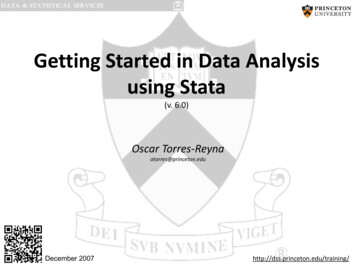
Regression: exploring relationshipsscatter csat percent02040% HS graduates taking SAT6080800800Mean composite SAT score9001000Mean composite SAT score900100011001100scatter csat high657075% adults HS diploma8085There seem to be a curvilinear relationship between csat and percent, and slightly linearbetween csat and high. To deal with U-shaped curves we need to add a square version ofthe variable, in this case percent squaregenerate percent2 percent 212PU/DSS/OTR
Regression: functional form/linearityThe command acprplot (augmented component-plus-residual plot) provides another graphical way to examine therelationship between variables. It does provide a good testing for linearity. Run this command after running aregressionregress csat percent high /* Notice we do not include percent2 */acprplot percent, lowessacprplot high, lowessacprplot high, lowess-250450Augmented component plus residual-200-150-100-50Augmented component plus residual5005500600acprplot percent, lowess02040% HS graduates taking SAT6080657075% adults HS diploma8085The option lowess (locally weighted scatterplot smoothing) draw the observed pattern in the data to help identifynonlinearities. Percent shows a quadratic relation, it makes sense to add a square version of it. High shows apolynomial pattern as well but goes around the regression line (except on the right). We could keep it as is for now.The model is:xi: regress csat expense percent percent2 income high college i.region, robustForm more details see apter2/statareg2.htm, and/or type help acprplot and help lowess.13PU/DSS/OTR
Regression: modelsxi: regress csat expense percent percent2 income high college i.region, robusteststo model4esttab, r2 ar2 se scalar(rmse). esttab, r2 ar2 se 931)college2.031(2.114 )4.671**(1.600)3.418**(1.145)Iregion 269.45***(18.00)5.077(20.75)Iregion 325.40*(12.53)5.209(10.42)Iregion 434.58***(9.450)19.25*(8.110)percent2consNR-sqadj. 20159.81Standard errors in parentheses* p 0.05, ** p 0.01, *** p 114PU/DSS/OTR
Regression: getting predicted valuesHow good the model is will depend on how well it predicts Y, the linearity of the model and the behavior ofthe residuals.There are two ways to generate the predicted values of Y (usually called Yhat) given the model:Option A, using generate after running the regression:xi: regress csat expense percent percent2 income high college i.region, robustgenerate csat predict b[ cons] b[percent]*percent b[percent]*percent b[percent2]*percent2 b[high]*high Option B, using predict immediately after running the regression:xi: regress csat expense percent percent2 income high college i.region, robustpredict csat predictlabel variable csat predict "csat predicted". predict csat predict(option xb assumed; fitted values)(1 missing value generated). label variable csat predict "csat predicted"15PU/DSS/OTR
Regression: observed vs. predicted valuesFor a quick assessment of the model run a scatter plot800Mean composite SAT score90010001100scatter csat csat predict850900950csat predicted10001050We should expect a 45 degree pattern in the data. Y-axis is the observed data and x-axis the predicteddata (Yhat).In this case the model seems to be doing a good job in predicting csat16PU/DSS/OTR
Regression: testing for homoskedasticityAn important assumption is that the variance in the residuals has to be homoskedastic or constant. Residualscannot varied for lower of higher values of X (i.e. fitted values of Y since Y Xb). A definition:“The error term [e] is homoskedastic if the variance of the conditional distribution of [ei] given Xi [var(ei Xi)], is constant fori 1 n, and in particular does not depend on x; otherwise, the error term is heteroskedastic” (Stock and Watson, 2003,p.126)When plotting residuals vs. predicted values (Yhat) we should not observe any pattern at all. In Stata we do thisusing rvfplot right after running the regression, it will automatically draw a scatterplot between residuals andpredicted values.Residuals02040rvfplot, yline(0)-40-20Residuals seem to slightlyexpand at higher levels ofYhat.850900950Fitted values1000105017PU/DSS/OTR
Regression: testing for homoskedasticityA non-graphical way to detect heteroskedasticiy is the Breusch-Pagan test. The null hypothesis is thatresiduals are homoskedastic. In the example below we fail to reject the null at 95% and concluded thatresiduals are homogeneous. However at 90% we reject the null and conclude that residuals are nothomogeneous.estat hettest. estat hettestBreusch-Pagan / Cook-Weisberg test for heteroskedasticityHo: Constant varianceVariables: fitted values of csatchi2(1)Prob chi2 2.720.0993The graphical and the Breush-Pagan test suggest the possible presence of heteroskedasticity in our model. Theproblem with this is that we may have the wrong estimates of the standard errors for the coefficients andtherefore their t-values.There are two ways to deal with this problem, one is using heteroskedasticity-robust standard errors, the otherone is using weighted least squares (see Stock and Watson, 2003, chapter 15). WLS requires knowledge of theconditional variance on which the weights are based, if this is known (rarely the case) then use WLS. In practiceit is recommended to use heteroskedasticity-robust standard errors to deal with heteroskedasticity.By default Stata assumes homoskedastic standard errors, so we need to adjust our model to account forheteroskedasticity. To do this we use the option robust in the regress command.xi: regress csat expense percent percent2 income high college i.region, robustFollowing Stock and Watson, as a rule-of-thumb, you should always assume heteroskedasticiy in your model18(see Stock and Watson, 2003, chapter 4) .PU/DSS/OTR
Regression: omitted-variable testHow do we know we have included all variables we need to explain Y?Testing for omitted variable bias is important for our model since it is related to the assumption that the errorterm and the independent variables in the model are not correlated (E(e X) 0)If we are missing variables in our model and “is correlated with the included regressor” and, “ the omitted variable is a determinant of the dependent variable” (Stock and Watson, 2003, p.144), then our regression coefficients are inconsistent.In Stata we test for omitted-variable bias using the ovtest command:xi: regress csat expense percent percent2 income high college i.region, robustovtest. ovtestRamsey RESET test using powers of the fitted values of csatHo: model has no omitted variablesF(3, 37) 1.25Prob F 0.3068The null hypothesis is that the model does not have omitted-variables bias, the p-value is higher than theusual threshold of 0.05 (95% significance), so we fail to reject the null and conclude that we do not needmore variables.19PU/DSS/OTR
Regression: specification errorAnother command to test model specification is linktest. It basically checks whether we need morevariables in our model by running a new regression with the observed Y (csat) against Yhat(csat predicted or Xβ) and Yhat-squared as independent variables1.The thing to look for here is the significance of hatsq. The null hypothesis is that there is nospecification error. If the p-value of hatsq is not significant then we fail to reject the null andconclude that our model is correctly specified. Type:xi: regresslinktestcsat expense percent percent2 income high college i.region, robust. td. Err.1.50184.0007885712.388t0.76-0.10-0.10Number of obsF( 2,47)Prob FR-squaredAdj R-squaredRoot MSEP t 0.4500.9230.924 50370.900.00000.94040.937916.431[95% Conf. 011364.446For more details see apter2/statareg2.htm, and/or type help linktest.20PU/DSS/OTR
Regression: multicollinearityAn important assumption for the multiple regression model is that independent variables are not perfectlymulticolinear. One regressor should not be a linear function of another.When multicollinearity is present standand errors may be inflated. Stata will drop one of the variables to avoida division by zero in the OLS procedure (see Stock and Watson, 2003, chapter 5).The Stata command to check for multicollinearity is vif (variance inflation factor). Right after running theregression type:. vifVariableVIF1/VIFpercent2percentIregion 2incomeIregion 3highcollegeexpenseIregion 1110.467506Mean VIF17.04A vif 10 or a 1/vif 0.10 indicates trouble.We know that percent and percent2 are related since one is the square of the other. They are ok since percenthas a quadratic relationship with Y, but this would be an example of multicolinearity.The rest of the variables look ok.Form more details see apter2/statareg2.htm, and/or type help vif.21PU/DSS/OTR
Regression: outliersTo check for outliers we use the avplots command (added-variable plots). Outliers are data pointswith extreme values that could have a negative effect on our estimators. After running the regressiontype:avplot expense-40-100-20-50e( csat X )0e( csat X )0205040100avplot percent-10-50e( percent X )5coef -5.9452674, (robust) se .64055286, t -9.2810-2000-10000e( expense X )10002000coef .00141156, (robust) se .00371641, t .38These plots regress each variable against all others, notice the coefficients on each. All data pointsseem to be in range, no outliers observed.For more details and tests on this and influential and leverage variables please eg/chapter2/statareg2.htmAlso type help diagplots in the Stata command window.22PU/DSS/OTR
Regression: outliers-2000 -100001000e( expense X )2000coef .00141156, (robust) se .00371641, t .38-505e( percent X )10-10-505e( income X )10-6-4-202e( high X )4-.4-.20.2e( Iregion 2 X ).4coef 5.0765963, (robust) se 20.753948, t .240e( percent2 X )500coef .0460468, (robust) se .01019105, t 4.5-5coef 1.8691679, (robust) se .93111302, t 2.010e( college X )5coef 3.4175732, (robust) se 1.1450333, t 2.e( csat X 40)-40-200 20e( csat X )-40-20 0 20 40e( csatX )40-40-200 20coef -.9143708, (robust) se .97326373, t -.94-500coef -5.9452674, (robust) se .64055286, t -9.28e( csat X40)-40-200 20e( csatX )40-40-200 20e( csat-40-200 20 X40) 60-10e( csatX )40-40-200 20e( csatX )40-40-200 20e( csatX )100-100-500 50avplots-.50e( Iregion 3 X ).5coef 5.2088169, (robust) se 10.422781, t .5-.50e( Iregion 4 X ).5coef 19.245404, (robust) se 8.1097615, t 2.23PU/DSS/OTR
Regression: summary of influence indicatorsIn SPSS: Analyze-RegressionLinear; click Save. Select under“Influence Statistics” to add as areg y x1 x2 x3new variable (DFB1 1) or insyntax typedfbeta x1Measures the influence ofREGRESSIONA case is an influential outliereach observation on the/MISSING LISTWISEifNote: you could also type:coefficient of a particular/STATISTICS COEFF OUTSindependent variable (forR ANOVA DfBeta 2/SQRT(N)predict DFx1, dfbeta(x1)example, x1). This is in/CRITERIA PIN(.05)POUT(.10)standard errors terms.Where N is the sample size. To estimate the dfbetas for all predictors just /NOORIGINtype:/DEPENDENT YAn observation is influential ifNote: Stata estimates/METHOD ENTER X1 X2 X3it has a significant effect ondfbetastandardized DfBetas./CASEWISE PLOT(ZRESID)the coefficient.OUTLIERS(3) DEFAULTSTo flag the cutoffDFBETA/SAVE MAHAL COOK LEVERgen cutoffdfbeta abs(DFx1) DFBETA SDBETA DFFIT2/sqrt(e(N)) & e(sample)SDFIT COVRATIO .In Stata type:DfBetaIndicator of leverage andhigh residuals.DfFitCovariance ratioHigh influence ifMeasures how much an DfFIT 2*SQRT(k/N)observation influences theregression model as a whole.Where k is the number ofparameters (including theHow much the predictedintercept) and N is thevalues change as a result ofsample size.including and excluding aparticular observation.Measures the impact of anobservation on the standarderrorsHigh impact if COVRATIO-1 3*k/NWhere k is the number ofparameters (including theintercept) and N is thesample size.After running the regression type:predict dfits if e(sample), dfitsTo generate the flag for the cutoff type:Same as DfBeta above (DFF 1)gen cutoffdfit abs(dfits) 2*sqrt((e(df m) 1)/e(N)) & e(sample)In Stata after running the regression typepredict covratio if e(sample),covratioSame as DfBeta above(COV 1)24PU/DSS/OTR
Regression: summary of distance measuresCook’s distanceMeasures how much anobservation influences theoverall model or predictedvalues.High influence ifD 4/NIn Stata after running theregression type:Where N is the sample size.It is a summary measure ofA D 1 indicates big outlierleverage and high residuals.problem.predict D, cooksdIn SPSS: Analyze-Regression-Linear;click Save. Select under “Distances”to add as a new variable (COO 1) orin syntax typeREGRESSION/MISSING LISTWISE/STATISTICS COEFF OUTS RANOVA/CRITERIA PIN(.05) POUT(.10)/NOORIGIN/DEPENDENT Y/METHOD ENTER X1 X2 X3/CASEWISE PLOT(ZRESID)OUTLIERS(3) DEFAULTS DFBETA/SAVE MAHAL COOK LEVERDFBETA SDBETA DFFIT SDFITCOVRATIO.High influence ifleverage h 2*k/NLeverageMeasures how much anobservation influencesregression coefficients.Where k is the number ofparameters (including theintercept) and N is the sample size.In Stata after running theregression type:Same as above (LEV 1)predict lev, leverageA rule-of-thumb: Leverage goesfrom 0 to 1. A value closer to 1 orover 0.5 may indicate problems.It is rescaled measure ofleverage.Mahalanobis distanceM leverage*(N-1)Where N is sample size.Higher levels indicate higherdistance from average values.The M-distance follows a Chisquare distribution with k-1 df andalpha 0.001 (where k is thenumber of independent variables).Any value over this Chi-squarevalue may indicate problems.Not availableSame as above (MAH 1)25PU/DSS/OTR
Sources for the summary tables:influence indicators and distance measures 65/regress.htm#outlier2 An Introduction to Econometrics Using Stata/Christopher F. Baum, StataPress, 2006 Statistics with Stata (updated for version 9) / Lawrence Hamilton,Thomson Books/Cole, 2006 UCLA apter2/statareg2.htm26PU/DSS/OTR
Regression: testing for normalityAnother assumption of the regression model (OLS) that impact the validity of all tests (p, t and F) is that residuals behave‘normal’. Residuals (here indicated by the letter “e”) are the difference between the observed values (Y) and the predicted values(Yhat): e Y – Yhat.In Stata you type: predict e, resid. It will generate a variable called “e” (residuals).Three graphs will help us check for normality in the residuals: kdensity, pnorm and qnorm.kdensity e, normalA kernel density plot produces a kind of histogram for theresiduals, the option normal overlays a normal distribution tocompare. Here residuals seem to follow a normal distribution.Below is an example using histogram.Density.01 .015.02.025Kernel density estimate0.005.03histogram e, kdensity normal-200204060.02-40Kernel density estimateNormal densityDensityResidualsIf residuals do not follow a ‘normal’ pattern then you shouldcheck for omitted variables, model specification, linearity,functional forms. In sum, you may need to reassess yourmodel/theory. In practice normality does not represent much of aproblem when dealing with really big samples.0.01kernel epanechnikov, bandwidth 6.4865-40-200Residuals204027PU/DSS/OTR
Regression: testing for normalityQuintile-normal plots (qnorm) check for non-normality in theextremes of the data (tails). It plots quintiles of residuals vsquintiles of a normal distribution. Tails are a bit off the normal.Standardize normal probability plot (pnorm) checksfor non-normality in the middle range of residuals.Again, slightly off the line but looks ok.pnorm e-400.00-200.25Residuals020Normal F[(e-m)/s]0.500.75401.00qnorm e0.000.250.50Empirical P[i] i/(N 1)1.000.75-20-400Inverse Normal2040A non-graphical test is the Shapiro-Wilk test for normality. It tests the hypothesis that the distribution is norm
R-square shows the amount of variance of Y explained by X. In this case expenseexplains 22% of the variance in SAT scores. Lets run the regression: regress . csat expense, robust. Adj R. 2 (not shown here) shows the same as . R. 2. but adjusted by the # of cases and # of variables. When t