Transcription
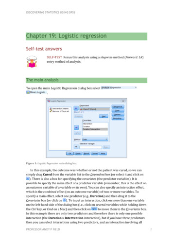
DISCOVERING STATISTICS USING SPSSChapter 19: Logistic regressionSelf-test answersSELF-TEST Rerun this analysis using a stepwise method (Forward: LR)entry method of analysis.The main analysisTo open the main Logistic Regression dialog box select.Figure 1: Logistic Regression main dialog boxIn this example, the outcome was whether or not the patient was cured, so we cansimply drag Cured from the variable list to the Dependent box (or select it and click on). There is also a box for specifying the covariates (the predictor variables). It ispossible to specify the main effect of a predictor variable (remember, this is the effect onan outcome variable of a variable on its own). You can also specify an interaction effect,which is the combined effect (on an outcome variable) of two or more variables. Tospecify a main effect, select one predictor (e.g., Duration) and then drag it to theCovariates box (or click on ). To input an interaction, click on more than one variableon the left-hand side of the dialog box (i.e., click on several variables while holding downthe Ctrl key, or Cmd on a Mac) and then click onto move them to the Covariates box.In this example there are only two predictors and therefore there is only one possibleinteraction (the Duration Intervention interaction), but if you have three predictorsthen you can select interactions using two predictors, and an interaction involving allPROFESSOR ANDY P FIELD1
DISCOVERING STATISTICS USING SPSSthree. In Figure 1, I have selected the two main effects of Duration, Intervention andthe Duration Intervention interaction. Select these variables too.Method of regressionYou can select a particular method of regression by clicking onand thenclicking on a method in the resulting drop-down menu. You were asked to do a forwardstepwise analysis so select the Forward: LR method of regression.Categorical predictorsSPSS needs to know which, if any, predictor variables are categorical. Click oninthe Logistic Regression dialog box to activate the dialog box in Figure 2. Notice that thecovariates are listed on the left-hand side, and there is a space on the right-hand side inwhich categorical covariates can be placed. Select any categorical variables you have (inthis example we have only one, so click on Intervention) and drag them to theCategorical Covariates box (or click on ).Figure 2: Defining categorical variables in logistic regressionLet’s use standard dummy coding (indicator) for this example. In our data, I coded‘cured’ as 1 and ‘not cured’ (our control category) as 0; therefore, select the contrast,then click onand thenso that the completed dialog box looks like Figure 2.Obtaining residualsTo save residuals click onsame options as in Figure 3.PROFESSOR ANDY P FIELDin the main Logistic Regression dialog box. Select the2
DISCOVERING STATISTICS USING SPSSFigure 3: Dialog box for obtaining residuals for logistic regressionFurther optionsFinally, click onin the main Logistic Regression dialog box to obtain the dialogbox in Figure 4. Select the same options as in the figure.Figure 4: Dialog box for logistic regression optionsInterpretationInitial outputOutput 1 tells both how we coded our outcome variable (it reminds us that 0 not curedand 1 cured) and how it has coded the categorical predictors (the parameter codingsfor Intervention). We chose indicator coding and so the coding is the same as the valuesin the data editor (0 no treatment, 1 treatment). If deviation coding had been chosenthen the coding would have been 1 (treatment) and 1 (no treatment). With a simplecontrast, ifhad been selected as the reference category the codes would havebeen 0.5 (Intervention no treatment) and 0.5 (Intervention treatment). and ifPROFESSOR ANDY P FIELD3
DISCOVERING STATISTICS USING SPSShad been selected as the reference category then the value of the codes wouldhave been the same but with their signs reversed. The parameter codes are importantfor calculating the probability of the outcome variable (P(Y)), but we will come to thatlater.Output 1For this first analysis we requested a forward stepwise method1 and so the initialmodel is derived using only the constant in the regression equation. Output 2 tells usabout the model when only the constant is included (i.e., all predictor variables areomitted). The table labelled Iteration History tells us that the log-likelihood of thisbaseline model is 154.08. This represents the fit of the most basic model to the data.When including only the constant, the computer bases the model on assigning everyparticipant to a single category of the outcome variable. In this example, SPSS can decideeither to predict that the patient was cured, or that every patient was not cured. It couldmake this decision arbitrarily, but because it is crucial to try to maximize how well themodel predicts the observed data, SPSS will predict that every patient belongs to thecategory in which most observed cases fell. In this example there were 65 patients whowere cured, and only 48 who were not cured. Therefore, if SPSS predicts that everypatient was cured then this prediction will be correct 65 times out of 113 (i.e., about58% of the time). However, if SPSS predicted that every patient was not cured, then thisprediction would be correct only 48 times out of 113 (42% of the time). As such, of thetwo available options it is better to predict that all patients were cured because thisresults in a greater number of correct predictions. The output shows a contingency tablefor the model in this basic state. You can see that SPSS has predicted that all patients arecured, which results in 0% accuracy for the patients who were not cured, and 100%accuracy for those observed to be cured. Overall, the model correctly classifies 57.5% ofpatients.Actually, this is a really bad idea when you have an interaction term because to look at an interaction youneed to include the main effects of the variables in the interaction term. I chose this method only to illustratehow stepwise methods work.1PROFESSOR ANDY P FIELD4
DISCOVERING STATISTICS USING SPSSOutput 2Output 3 summarizes the model (Variables in the Equation), and at this stage thisentails quoting the value of the constant (b0), which is equal to 0.30. The table labelledVariables not in the Equation tells us that the residual chi-square statistic is 9.83 which issignificant at p .05 (it labels this statistic Overall Statistics). This statistic tells us thatthe coefficients for the variables not in the model are significantly different from zero –in other words, that the addition of one or more of these variables to the model willsignificantly affect its predictive power. If the probability for the residual chi-square hadbeen greater than .05 it would have meant that forcing all of the variables excluded fromthe model into the model would not have made a significant contribution to itspredictive power.The remainder of this table lists each of the predictors in turn, with a value of Roa’sefficient score statistic for each one (column labelled Score). In large samples when thenull hypothesis is true, the score statistic is identical to the Wald statistic and thelikelihood ratio statistic. It is used at this stage of the analysis because it iscomputationally less intensive than the Wald statistic and so can still be calculated insituations when the Wald statistic would prove prohibitive. Like any test statistic, Roa’sscore statistic has a specific distribution from which statistical significance can beobtained. In this example, Intervention and the Intervention Duration interactionboth have significant score statistics at p .01 and could potentially make a contributionto the model, but Duration alone does not look likely to be a good predictor because itsscore statistic is non-significant, p .05. As mentioned earlier, the stepwise calculationsare relative and so the variable that will be selected for inclusion is the one with thehighest value for the score statistic that has a significance below .05. In this example,that variable will be Intervention because its score statistic (9.77) is the biggest.PROFESSOR ANDY P FIELD5
DISCOVERING STATISTICS USING SPSSOutput 3Step 1: InterventionAs I predicted in the previous section, whether or not an intervention was given to thepatient (Intervention) is added to the model in the first step. As such, a patient is nowclassified as being cured or not based on whether they had an intervention or not(waiting list). This can be explained easily if we look at the crosstabulation for thevariables Intervention and Cured. The model will use whether a patient had anintervention or not to predict whether they were cured or not by applying thecrosstabulation table shown in Table 1.Table 1: Crosstabulation of intervention with outcome status (cured or not)Intervention or Not (Intervention)Cured? (Cured)No TreatmentInterventionNot Cured3216Cured2441Total5657The model predicts that all of the patients who had an intervention were cured.There were 57 patients who had an intervention, so the model predicts that these 57patients were cured; it is correct for 41 of these patients, but misclassifies 16 people as‘cured’ who were not cured – see Table 1. In addition, this new model predicts that all ofthe 56 patients who received no treatment were not cured; for these patients the modelis correct 32 times but misclassifies as ‘not cured’ 24 people who were.PROFESSOR ANDY P FIELD6
DISCOVERING STATISTICS USING SPSSOutput 4Output 4 shows summary statistics about the new model (which we’ve already seencontains Intervention). The overall fit of the new model is assessed using the loglikelihood statistic. In SPSS, rather than reporting the log-likelihood itself, the value ismultiplied by 2 (and sometimes referred to as 2LL): this multiplication is donebecause 2LL has an approximately chi-square distribution and so it makes it possibleto compare values against those that we might expect to get by chance alone. Rememberthat large values of the log-likelihood statistic indicate poorly fitting statistical models.At this stage of the analysis the value of 2LL should be less than the value when onlythe constant was included in the model (because lower values of 2LL indicate that themodel is predicting the outcome variable more accurately). When only the constant wasincluded, 2LL 154.08, but now Intervention has been included this value has beenreduced to 144.16. This reduction tells us that the model is better at predicting whethersomeone was cured than it was before Intervention was added. The question of howmuch better the model predicts the outcome variable can be assessed using the modelchi-square statistic, which measures the difference between the model as it currentlystands and the model when only the constant was included. We can assess thesignificance of the change in a model by taking the log-likelihood of the new model andsubtracting the log-likelihood of the baseline model from it. The value of the model chisquare statistic works on this principle and is, therefore, equal to 2LL withIntervention included minus the value of 2LL when only the constant was in themodel (154.08 144.16 9.92). This value has a chi-square distribution and so itsstatistical significance can be calculated easily.2 In this example, the value is significantThe degrees of freedom will be the number of parameters in the new model (the number of predictors plus1, which in this case with one predictor, means 2) minus the number of parameters in the baseline model(which is 1, the constant). So, in this case, df 2 – 1 1.2PROFESSOR ANDY P FIELD7
DISCOVERING STATISTICS USING SPSSat the .05 level and so we can say that overall the model is predicting whether a patientis cured or not significantly better than it was with only the constant included. Themodel chi-square is an analogue of the F-test for the linear regression. In an ideal worldwe would like to see a non-significant overall 2LL (indicating that the amount ofunexplained data is minimal) and a highly significant model chi-square statistic(indicating that the model including the predictors is significantly better than withoutthose predictors). However, in reality it is possible for both statistics to be highlysignificant.There is a second statistic called the step statistic that indicates the improvement inthe predictive power of the model since the last stage. At this stage there has been onlyone step in the analysis and so the value of the improvement statistic is the same as themodel chi-square. However, in more complex models in which there are three or fourstages, this statistic gives a measure of the improvement of the predictive power of themodel since the last step. Its value is equal to 2LL at the current step minus 2LL at theprevious step. If the improvement statistic is significant then it indicates that the modelnow predicts the outcome significantly better than it did at the last step, and in aforward regression this can be taken as an indication of the contribution of a predictorto the predictive power of the model. Similarly, the block statistic provides the change in 2LL since the last block (for use in hierarchical or blockwise analyses).Output 4 also tells us the values of Cox and Snell’s and Nagelkerke’s R2, but we willdiscuss these a little later. There is also a classification table that indicates how well themodel predicts group membership; because the model is using Intervention to predictthe outcome variable, this classification table is the same as Table 1. The current modelcorrectly classifies 32 patients who were not cured but misclassifies 16 others (itcorrectly classifies 66.7% of cases). The model also correctly classifies 41 patients whowere cured but misclassifies 24 others (it correctly classifies 63.1% of cases). Theoverall accuracy of classification is, therefore, the weighted average of these two values(64.6%). So, when only the constant was included, the model correctly classified 57.5%of patients, but now, with the inclusion of Intervention as a predictor, this has risen to64.6%.Output 5The next part of the output (Output 5) is crucial because it tells us the estimates forthe coefficients for the predictors included in the model. This section of the output givesus the coefficients and statistics for the variables that have been included in the model atthis point (namely Intervention and the constant). The b-value is the same as the bvalue in linear regression: they are the values that we need to replace in the regressionPROFESSOR ANDY P FIELD8
DISCOVERING STATISTICS USING SPSSequation to establish the probability that a case falls into a certain category. We saw inlinear regression that the value of b represents the change in the outcome resulting froma unit change in the predictor variable. The interpretation of this coefficient in logisticregression is very similar in that it represents the change in the logit of the outcomevariable associated with a one-unit change in the predictor variable. The logit of theoutcome is simply the natural logarithm of the odds of Y occurring.The crucial statistic is the Wald statistic3 which has a chi-square distribution and tellsus whether the b coefficient for that predictor is significantly different from zero. If thecoefficient is significantly different from zero then we can assume that the predictor ismaking a significant contribution to the prediction of the outcome (Y). The Wald statisticshould be used cautiously because when the regression coefficient (b) is large, thestandard error tends to become inflated, resulting in the Wald statistic beingunderestimated (see Menard, 1995). However, for these data it seems to indicate thathaving the intervention (or not) is a significant predictor of whether the patient is cured(note that the significance of the Wald statistic is less than .05).You should notice that the odds ratio is what SPSS reports as Exp(B). The odds ratiois the change in odds; if the value is greater than 1 then it indicates that as the predictorincreases, the odds of the outcome occurring increase. Conversely, a value less than 1indicates that as the predictor increases, the odds of the outcome occurring decrease. Inthis example, we can say that the odds of a patient who is treated being cured are 3.41times higher than those of a patient who is not treated.In the options, we requested a confidence interval for the odds ratio and it can alsobe found in the output. As with any confidence interval it is computed such that if wecalculated confidence intervals for the value of the odds ratio in 100 different samples,then these intervals would include value of the odds ratio in the population in 95 ofthose samples. Assuming the current sample is one of the 95 for which the confidenceinterval contains the true value, then we know that the population value of the oddsratio lies between 1.56 and 7.48. However, our sample could be one of the 5% thatproduces a confidence interval that ‘misses’ the population value.The important thing about this confidence interval is that it doesn’t cross 1 (bothvalues are greater than 1). This is important because values greater than 1 mean that asthe predictor variable increases, so do the odds of (in this case) being cured. Values lessthan 1 mean the opposite: as the predictor variable increases, the odds of being cureddecrease. The fact that both limits of our confidence interval are above 1 gives usconfidence that the direction of the relationship that we have observed is true in thepopulation (i.e. it’s likely that having an intervention compared to not increases the oddsof being cured). If the lower limit had been below 1 then it would tell us that there is achance that in the population the direction of the relationship is the opposite to what weAs we have seen, this is simply b divided by its standard error (1.229/0.40 3.0725); however, SPSSactually quotes the Wald statistic squared. For these data 3.0725 2 9.44 as reported (within roundingerror) in the table.3PROFESSOR ANDY P FIELD9
DISCOVERING STATISTICS USING SPSShave observed. This would mean that we could not trust that our intervention increasesthe odds of being cured.Output 6The test statistics for Intervention if it were removed from the model are in Output6. Now, remember that earlier on I said how the regression would place variables intothe equation and then test whether they then met a removal criterion. Well, the Model ifTerm Removed part of the output tells us the effects of removal. The important thing tonote is the significance value of the log-likelihood ratio. The log-likelihood ratio for thismodel is significant (p .01) which tells us that removing Intervention from the modelwould have a significant effect on the predictive ability of the model – in other words, itwould be a very bad idea to remove it!Finally, we are told about the variables currently not in the model. First of all, theresidual chi-square (labelled Overall Statistics in the output), which is non-significant,tells us that none of the remaining variables have coefficients significantly different fromzero. Furthermore, each variable is listed with its score statistic and significance value,and for both variables their coefficients are not significantly different from zero (as canbe seen from the significance values of .964 for Duration and .835 for theDuration Intervention interaction). Therefore, no further variables will be added tothe model.SELF-TEST Calculate the values of Cox and Snell’s and Nagelkerke’s R2reported by SPSS. (Remember the sample size, N, is 113.)Cox and Snell’s R2 is calculated from this equation:SPSS reports 2LL(new) as 144.16 and 2LL(baseline) as 154.08. The sample size, N, is113. SoPROFESSOR ANDY P FIELD10
DISCOVERING STATISTICS USING SPSSNagelkerke’s adjustment is calculated from:SELF-TEST Use the case summaries function in SPSS to create a table forthe first 15 cases in the file Eel.sav showing the values of Cured,Intervention, Duration, the predicted probability (PRE 1) and thepredicted group membership (PGR 1) for each case.The completed dialog box should look like this:Figure 5PROFESSOR ANDY P FIELD11
DISCOVERING STATISTICS USING SPSSSELF-TEST Conduct a hierarchical logistic regression analysis on thesedata. Enter Previous and PSWQ in the first block and Anxious in thesecond (forced entry).Running the analysis: block entry regressionTo run the analysis, we must first bring up the main Logistic Regression dialog box, byselecting. In this example, we know of twopreviously established predictors and so it is a good idea to enter these predictors intothe model in a single block. Then we can add the new predictor in a second block (bydoing this we effectively examine an old model and then add a new variable to thismodel to see whether the model is improved). This method is known as block entry andFigure 6 shows how it is specified.It is easy to do block entry regression. First you should use the mouse to select thevariable scored from the variables list and then transfer it to the box labelled Dependentby clicking on . Second, you should select the two previously established predictors.So, select PSWQ and Previous from the variables list and transfer them to the boxlabelled Covariates by clicking on . Our first block of variables is now specified. Tospecify the second block, click onto clear the Covariates box, which should now belabelled Block 2 of 2. Now select Anxious from the variables list and transfer it to thebox labelled Covariates by clicking on . We could at this stage select some interactionsto be included in the model, but unless there is a sound theoretical reason for believingthat the predictors should interact there is no need. Make sure that Enter is selected asthe method of regression (this method is the default and so should be selected already).Once the variables have been specified, you should select the options described in thechapter, but because none of the predictors are categorical there is no need to use theoption. When you have selected the options and residuals that you want youcan return to the main Logistic Regression dialog box and click on.PROFESSOR ANDY P FIELD12
DISCOVERING STATISTICS USING SPSSFigure 6The output of the logistic regression will be arranged in terms of the blocks that werespecified. In other words, SPSS will produce a regression model for the variablesspecified in block 1, and then produce a second model that contains the variables fromboth blocks 1 and 2.First, the output shows the results from block 0: the output tells us that 75 cases havebeen accepted, and that the dependent variable has been coded 0 and 1 (because thisvariable was coded as 0 and 1 in the data editor, these codings correspond exactly to thedata in SPSS). We are then told about the variables that are in and out of the equation. Atthis point only the constant is included in the model, and so to be perfectly honest noneof this information is particularly interesting!PROFESSOR ANDY P FIELD13
DISCOVERING STATISTICS USING SPSSDependent Variable EncodingOriginal ValueInternal ValueMissed Penalt y0Scored Penalt y1Output 7Classification Tablea,bPredic tedStep 0Obs erv edRes ult of PenaltyKickMissed PenaltyScored PenaltyRes ult of Penalty KickMissedScoredPenalt yPenalt y035040Ov erall PercentagePercentageCorrect.0100.053. 3a. Constant is included in the model.b. The cut v alue is . 500Variables in the Equati onStep 0ConstantB.134S.E.231Wald.333dfSig.5641Exp(B)1. 143Variables not in the EquationStep0VariablesOv erall St atist icsPREVIOUSPSWQScore34. 10934. 19341. 558df112Sig.000.000.000Output 8The results from block 1 are shown next, and in this analysis we forced SPSS to enterPrevious and PSWQ into the regression model. Therefore, this part of the outputprovides information about the model after the variables Previous and PSWQ havebeen added. The first thing to note is that 2LL is 48.66, which is a change of 54.98(which is the value given by the model chi-square). This value tells us about the model asa whole, whereas the block tells us how the model has improved since the last block. Thechange in the amount of information explained by the model is significant (p .001), andso using previous experience and worry as predictors significantly improves our abilityto predict penalty success. A bit further down, the classification table shows us that 84%of cases can be correctly classified using PSWQ and Previous.In the intervention example, Hosmer and Lemeshow’s goodness-of-fit test was 0. Thereason is that this test can’t be calculated when there is only one predictor and thatpredictor is a categorical dichotomy! However, for this example the test can becalculated. The important part of this test is the test statistic itself (7.93) and thesignificance value (.3388). This statistic tests the hypothesis that the observed data aresignificantly different from the predicted values from the model. So, in effect, we want anon-significant value for this test (because this would indicate that the model does notdiffer significantly from the observed data). We have a non-significant value here, whichis indicative of a model that is predicting the real-world data fairly well.PROFESSOR ANDY P FIELD14
DISCOVERING STATISTICS USING SPSSThe part of the output labelled Variables in the Equation then tells us the parametersof the model when Previous and PSWQ are used as predictors. The significance valuesof the Wald statistics for each predictor indicate that both PSWQ and Previoussignificantly predict penalty success (p .01). The value of the odds ratio (Exp(B)) forPrevious indicates that if the percentage of previous penalties scored goes up by one,then the odds of scoring a penalty also increase (because the odds ratio is greater than1). The confidence interval for this value ranges from 1.02 to 1.11, so we can be veryconfident that the value of the odds ratio in the population lies somewhere betweenthese two values. What’s more, because both values are greater than 1 we can also beconfident that the relationship between Previous and penalty success found in thissample is true of the whole population of footballers. The odds ratio for PSWQ indicatesthat if the level of worry increases by one point along the Penn State worry scale, thenthe odds of scoring a penalty decrease (because it is less than 1). The confidence intervalfor this value ranges from .68 to .93 so we can be very confident that the value of theodds ratio in the population lies somewhere between these two values. In addition,because both values are less than 1 we can be confident that the relationship betweenPSWQ and penalty success found in this sample is true of the whole population offootballers. If we had found that the confidence interval ranged from less than 1 to morethan 1, then this would limit the generalizability of our findings because the odds ratioin the population could indicate either a positive (odds ratio 1) or negative (odds ratio 1) relationship.A glance at the classification plot also brings us good news because most cases areclustered at the ends of the plot and few cases lie in the middle of the plot. Thisreiterates what we know already: that the model is correctly classifying most cases. Wecan, at this point, also calculate R2 by dividing the model chi-square by the original valueof –2LL. The result is:R2 model chi-square54.977 .53original 2 LL103.6385We can interpret the result as meaning that the model can account for 53% of thevariance in penalty success (so, roughly half of what makes a penalty kick successful isstill unknown).PROFESSOR ANDY P FIELD15
DISCOVERING STATISTICS USING SPSSOmni bus Tests of Model Coeffici entsStep 1StepBlockModelChi-square54. 97754. 97754. 977df222Sig.000.000.000Model SummaryStep1-2 Loglikelihood48. 662Cox & SnellR Square.520NagelkerkeR Square.694Hosmer and Lemeshow TestStep1Chi-square7.931df7Sig.339Contingency Tabl e for Hosmer and Lemeshow TestStep1123456789Res ult of Penalty Kick Missed PenaltyObs erv ed Expec ted87. 90487. 77986. 70545. 43823. 94521. 82021. 0041.2980.108Res ult of Penalty Kick Scored PenaltyObs erv ed Expec ted0.0960.22101. 29542. 56264. 05566. 18066. 99677. 7021110. 892Tot al8888888811Classification TableaPredic tedStep 1Obs erv edRes ult of PenaltyKickRes ult of Penalty KickMissedScoredPenalt yPenalt y305733Missed PenaltyScored PenaltyOv erall PercentagePercentageCorrect85. 782. 584. 0a. The cut v alue is . 500Variables in the EquationStepa1PREVI OUSPSWQConstantB.065-. 2301. 280S.E.022.0801. 670Wald8. 6098. 309.588df111Sig.003.004.443Exp(B)1. 067.7943. 59895. 0% C.I .f or EXP(B)LowerUpper1. 0221. 114.679.929a. Variable(s) ent ered on st ep 1: PREVI OUS, PSWQ.Output 9PROFESSOR ANDY P FIELD16
DISCOVERING STATISTICS USING SPSSOutput 10The output for block 2 shows what happens to the model when our new predictor isadded (Anxious). So, we begin with the model that we had in block 1 and we addAnxious to it. The effect of adding Anxious to the model is to reduce –2LL to 47.416 (areduction of 1.246 from the model in block 1 as shown in the model chi-square and blockstatistics). This improvement is non-significant, which tells us that including Anxious inthe model has not significantly improved our ability to predict whether a penalty will bescored or missed. The classification table tells us that the model is now correctlyclassifying 85.33% of cases. Remember that in block 1 there were 84% correctlyclassified and so an extra 1.33% of cases are now classified (not a great deal more – infact, examining the table shows us that only one extra case has now been correctlyclassified).The table labelled Variables in the Equation now contains all three predictors andsomething very interesting has happened: PSWQ is still a significant predictor ofpenalty success;
prediction would be correct only 48 times out of 113 (42% of the time). As such, of the two available options it is better to predict that all patients were cured because this results in a gr