Transcription
Monte Carlo Simulationin EngineeringMikael AmelinDraft versionKTH Royal Institute of TechnologyElectric Power SystemsStockholm 2013
PREFACEThis compendium describes how Monte Carlo methods can be applied to simulate technical systems.The description covers background on probability theory and random number generation as well as thethoery and practice of efficient Monte Carlo simulations. The core of the compendium is based on lectures that have been given at KTH for several years; however, the presentation here also includes moreexplanatory texts and exercises with solutions.I would like to give a warm thank you to colleagues and students who have helped improve the contents of this compendium by asking questions, pointing out errors and suggesting additional topics.StockholmAugust 2015Mikael Ameliniii
iv
CONTENTSPreface . iiiContents . v1 Introduction . 11.1 Brief History . 11.2 Problem Definition . 11.3 Notation . 52 Random Variables . 72.1 Probability Distributions . 72.1.1 Populations . 72.1.2 Other Common Definitions of Probability Distributions . 82.2 Statistical Properties . 102.3 Arithmetics of Random Variables . 14Exercises . 153 Random Numbers . 173.1 Pseudo-random Numbers . 173.2 Transformation of Random Numbers . 193.2.1 Independent Random Numbers . 193.2.2 Correlated Random Numbers . 20Exercises . 214 Simple Sampling . 254.1 Estimating Expectation Values . 254.2 Other Estimates . 294.3 Application . 30Exercises . 315 Variance Reduction Techniques . 335.1 Complementary Random Numbers . 335.1.1 Principle . 335.1.2 Application . 345.2 Dagger Sampling . 365.2.1 Principle . 365.2.2 Application . 375.3 Control Variates . 375.3.1 Principle . 375.3.2 Application . 375.4 Correlated Sampling . 385.4.1 Principle . 385.4.2 Application . 38v
5.5Importance Sampling .5.5.1 Principle .5.5.2 Application .5.6 Stratified Sampling .5.6.1 Principle .5.6.2 Application .Exercises .383839404042446 Efficient Monte Carlo Simulations . 556.1 Mathematical Model . 556.2 Choice of Simulation Method . 556.3 Testing . 55A Probability Distributions . 57B Akabuga District Simulation . 59B.1 Analysis of the System . 59B.2 Simulation Code . 62C Probabilistic Production Cost Simulation . 77Further reading . 77Solutions to Exercises . 79vi
Chapter 1INTRODUCTIONMonte Carlo methods refers to a class of methods to solve mathematical problems using random samples. A straightforward example is the computation of the expectation value of a random variable;instead of computing the expectation value according to the definition (which may involve solving complex integrals) we observe the behaviour of the random variable, i.e., we collect samples, and estimateits expactation value based on these samples. However, Monte Carlo methods may also be used for solving deterministic problems. This might seem odd at a first glance, but the idea is simply to find a random variable, the statistic properties of which is depending on the solution to the deterministic problem. An example of this would be an opinion poll. Assume that there is going to be an election. If weignore that people may change their preferences over time and consider just one specific point of timethen the share of voters who are planning to vote for a certain candidate is deterministic. However, inorder to compute the true value of this share, we would have to ask all voters which candidate theyfavour. An alternative would be to ask a limited number of randomly chosen voters and use these samples to estimate the share of votes the candidate will obtain.This compendium will describe how Monte Carlo methods can be used for simulation of various technical systems. The compendium includes many mathematical definitions and formulae, but it should beemphasised that this is not a mathematical textbook. The focus of the presentation will be how MonteCarlo methods can be applied to solve engineering problems; hence, the mathematics should be seen asa tool and not a topic in itself. This means that for example mathematical proofs will only be provided inorder to improve the understanding of the described methods, and some mathematical details might beignored.1.1Brief HistoryThe phrase “Monte Carlo methods” was coined in the beginning of the 20th century, and refers to thefamous casino in Monaco1—a place where random samples indeed play an important role. However,the origin of Monte Carlo methods is older than the casino.To be added: History of probability theory To be added: Bernouille, Poisson and the law of large numbers.To be added: Buffon’s needleTo be added: Modern development.1.2Problem DefinitionThis entire compendium is focusing on methods for simulation of systems on one specific format. (Thismight seem as a large limitation, but the reader will soon see that a wide range of systems fit into thisformat.) An overview of this format is given in figure 1.1. The studied systems are modelled by a set of1. It has been said that if Monte Carlo methods had been first explored today, they would have beenreferred to as “Las Vegas methods”.1.1 Brief History1
Chapter 1 IntroductionInputs, YFigure 1.1Model,g(Y)Outputs, XThe simulation problem considered in this compendium.random input variables, which we at this point simply collect into a vector, Y. The probability distribution of these inputs must be known. We also have and a set of output variables, which we also collectinto a vector, X. As these outputs are depending on the random inputs, they must be random variablesas well; however, the probability distribution of the outputs is not known—in fact, the objective of simulating the system is to determine the behaviour of the outputs. Finally, we have a mathematical modelof the system, which determines how the values of the outputs are calculated given the values of theinput variables. We denote the mathematical model as a function g, such that X g(Y). This functiondefines how the values of the outputs are computed given the values of the input values. In this compendium, a set of random values for each input will be referred to as a scenario.Example 1.1. To be added: Example of a model expressed explicitly.To be added: Discussion of model constants In example 1.1 it was possible to write the output as an explicit function of the input. This is however aspecial case, and most models g(Y) will be defined implicitly and may require several steps before theoutput values are computed. A typical example would be there the output values depend on the solutionto an optimisation problem, and also require a few other calculations to obtain the final results. forexample from the solution to an optimisation problem, as illustrated in the next example:Example 1.2 (simple two-area power system). Consider a power system divided in twoareas: a generation centre and a load centre. The generation centre is dominated by largerenewable power plants, but there is also a small local load, whereas the load centre hasmost of the load in the system, but there is also some thermal power plants. The renewablepower plants in the generation centre are assumed to have negligible variable operationcosts and the risk of outages is also negligible. Moreover, the capacity of the renewablepower plants is larger than the maximal local load; hence, the generation centre always hasexcess power to export to the load centre. However, the interconnection between the areashas a limited capacity and there is a risk of outages. There are also electrical losses on theinterconnection; these losses are proportional to the square of the power injected into theinterconnection. The variable costs of the thermal power plants in the load centre isassumed to be directly proportional to the power output (i.e., start-up costs and ramp ratesetc. may be neglected) and there is a risk of outages in these units. Finally, the load in thetwo areas is varying randomly. It can be assumed that the load is described by one probability distribution for the total load of the system, and another probability distribution forthe share of the load that is located in the main load centre.The system is operated in such a manner that the first priority is to avoid load shedding(i.e., when load has to be disconnected because there is not sufficient generation capacityavailable in the system) and the second priority is to minimise the generation costs. Voltage and frequency control may be neglected. The objective of simulating this power systemis to determine the total operation cost and the risk of load shedding. Formulate a model ofthis kind of power system and show how the values of the outputs are calculated given thevalues of the inputs.Solution: Start by introducing symbols for the inputs and outputs of this simulationproblem:InputsThe inputs are the random variables of the model. In this case we have random outages inthermal power plants and the interconnection between the areas, as well as random loadsin the two areas:21.2 Problem Definition
Chapter 1 IntroductioncDtotGgP share of the total load that is located in the main load centre,total load in the system,available generation capacity in thermal plants g,available transmission capacity on the interconnection between the two areas.OutputsWe are actually only interested in two outputs (the total operation cost and whether loadshedding occurs or not), but in order to compute these two values, we will need some partial results. Since the partial results also depend on the values of the random inputs, theywill in practice also be outputs (i.e., random variables with unknown probability distributions depending on the probability distributions of the inputs). In this case, the model willbe generating the following outputs:load in the main load centre,load in the generation centre,generation in thermal power plant g,generation in the renewable power plants,loss of load occasion (binary variable equal to 1 if load shedding is necessary and0 otherwise),P transmission from the generation centre to the load centre,TOC total operation cost,U unserved load,D1D2GgHLOLO where LOLO and TOC are the outputs that we want to study.Model constantsIn order to formulate the mathematical model, we are going to need some additional values: Gg variable operation cost of thermal power plant g, U penalty cost for unserved load, L loss coefficient for the interconnection between the areas,H available generation capacity in the renewable power plants.To be added: Comment the penalty cosst for unserved load Mathematical modelNow we can formulate the calculations necessary to compute the values of the outputs fora scenario. First, we need to compute the local load in each area:D1 c·Dtot,(1.1a)D2 (1 – c)·Dtot.(1.1b)The next step is to determine how the system will be operated. This can be formulated asan optimisation problem, where the objective function (1.2a) states that the costs of thesystem should be minimised, the constraints (1.2b), (1.2c) state that there should be balance between generation, load and import in the load centre and between generation, loadan export in the generation centre and the limits (1.2d)–(1.2g) state that generation andtransmission may not exceed the available capacity.minimise Gg Gg U U,(1.2a)gsubject to Gg P – P 2(1.2b) D 1 – U,gH D2 P,(1.2c)0 Gg G g , g,(1.2d)1.2 Problem Definition3
Chapter 1 Introduction0 H H,(1.2e)0 P P,(1.2f)0 U.(1.2g)To be added: Explanation of the model and description of how the problem can be solvedusing a simple algorithm Finally, once it has been determined how the power system is operated, the two main outputs can be computed from the solution to the optimisation problem: 0LOLO 1TOC if U 0,(1.3a)if U 0, Gg Gg .(1.3b)gIt is important to notice that the model g is deterministic! Hence, if we have two scenarios, y1 and y2,producing two sets of output values, x1 g(y1) and x2 g(y2) then if y1 y2 we will get that x1 x2. If thisproperty is not fulfilled, the model is missing inputs and should be reformulated, as in the followingexample:Example 1.3. To be added: Example of a model which is missing an input value (powergrid, where the reliability is depending on the sucess of reclosing breakers after a failure).Many of the examples in the following chapters of this compendium will be based on an system basedon the model from example 1.1. Additional details on this example system are collected in appendix B.Here, we will just introduce the system and identify the model constants:Example 1.4 (Akabuga District). Akabuga is a small town in East Africa. The town is notconnected to the national grid, but has a local system of its own. The local grid is suppliedby a 350 kW hydro power plant in Ekyaalo. The variable costs of the hydro power plant arenegligible and it can be considered to be 100% reliable. There is a 11 kV transmission linebetween Ekyaalo and Akabuga. This line has a maximal capacity of 300 kW, the reliabilityis 99% and the losses of the line are equal to 5·10–5P2, where P is the power injected on theEkyaalo side. In Akabuga proper, there are two diesel generator sets. The first unit has200 kW capacity, the variable costs are 10 /kWh and the availability is 90%. The secondunit has 150 kW capacity, the variable costs are 12 /kWh and the availability is 80%.The total load of the system is varying between 200 and 600 kW according to the probabilities listed in table 1.1. It is 50% probability that 85% of the total load is in Akabuga and 50%probability that 90% of the total load is in Akabuga.State the values of the model constants for a simulation of Akabuga District.Table 1.1 Probabilities of different load levels in Akabuga District.Total load [kW]Probability [ ]200203004040025500106005Solution: The model constants are the inputs that do not change value between scenarios. From the description above, we can identify the following model constants: G1 variable operation cost of the large diesel generator set 10, G1 variable operation cost of the small diesel generator set 12, L loss coefficient for the 11 kV transmission line 5·10–5,41.2 Problem Definition
Chapter 1 IntroductionH available generation capacity in the hydro power plant.The capacity of diesel generator sets and the transmission line which are mentioned aboveare also not changing between scenarios. However, due to the risk of outages, the availablecapacity (which is what needs to be considered in the simulation) is a random variable;hence, the maximal capacity will appear in the probability distribution of the inputs (cfexample 2.2).1.3NotationBefore we start investigating the application of Monte Carlo methods to solve the simulation problemdescribed above, it might be useful to introduce a general notation, which will be used throughout thiscompendium. Once the reader is familiar with this notation, it will be more straightforward to interpretthe mathematical expression appearing in the following chapters. Random variables. All random variables are denoted by upper-case Latin letters; usually justone single letter, for example Y or X, but sometimes several letters, such as LOLO and TOC inexample 1.2. Samples. An observation of a random variable (i.e., a sample) is denoted by the lower-case ofthe symbol used for the random variable itself, for example y or x. In most cases, we also use anindex in order to separate different samples from each other, i.e., yi or xi. Populations. A population is denoted by the same upper-case Latin letter as the correspondingrandom variable, but using a script font, for example Y or X. The value of the i:th unit in a population is denoted by the lower-case symbol used for population itself, indexed by i, for exampleyi or xi. Probability distributions. Probability distributions are denoted by Latin f in upper or lowercase (depending on interpretation2) and an index showing to which random variable the distribution is associated, for example fY or FX. The idea of the index is to tell different probabilitydistributions apart from each other. Statistical properties. Key statistical properties of a probability distribution are denoted bylower-case Greek letters and an index showing to which random variable the statistical property is associated, for example Y or X. The idea of the index is to tell different probability distributions apart from each other. Estimates. Estimates of key statistical properties for a probability distribution are denoted byupper or lower case (depending on interpretation3) Latin counterpart of the symbol used forthe statistical property itself and an index showing to which random variable the statisticalproperty is associated, for example MX or sX. The idea of the index is to tell different probabilitydistributions apart from each other.2. Cf. section 2.1.3. Cf. section 4.1.1.3 Notation5
Chapter 1 Introduction61.3 Notation
Chapter 2RANDOM VARIABLESAs the idea of Monte Carlo simulation is to estimate values using random observations, it is natural thata basic understanding of probability theory is necessary. This chapter summarises the probability theory that will be used in the remainder of the compendium. The focus of the presentation will be on random variables.2.1Probability DistributionsIntuitively, we may understand a random variable exactly as the name suggests, i.e., a variable, thevalue of which is varying according to some random pattern. This pattern, which characterises thebehaviour of the random variable is referred to as its probability distribution. There is an infinite number of possible probability distributions; however, some common classes of distributions have beenidentified and named. A brief overview can be found in appendix A.2.1.1PopulationsThe formal mathematical definition of a random variable is however slightly more complex, and willtherefore not be discussed here.For a discussion of sampling and Monte Carlo simulation, a useful interpretation of random variablesis to consider a random variable to be associated with a certain population, which we define as follows:Definition 2.1. The random variable X corresponds to a population, X, which is a set with Nmembers (which are referred to as “units”). Each unit has a value, xi, which may be multidimensional. The values of the units in X do not have to be unique, but they should includeall possible outcomes of the random variable X and the relative occurrence of a certainvalue should be proportional to the probability of the corresponding outcome.Example 2.1. State the population corresponding to the following random variables:a) D, which represents the result of throwing a normal six-sided dice.b) To be added Solution:a) D {1, 2, 3, 4, 5, 6}b) To be added Based on this definition we can distinguish between some main categories of populations (and consequently between different categories of random variables). First we can differentiate between variableswhere the outcome can only belong to specific, discrete values or if the outcome can be found in continuous intervals:Definition 2.2. If the population is finite or countable infinite, the random variable is dis2.1 Probability Distributions7
Chapter 2 Random Variablescrete; otherwise, it is continuous.To be added: Examples As pointed out in definition 2.1, the units in a population may have more than one value. If each unithas one value, the population directly corresponds to one random variable. However, if the units havemore than one value, we may consider each value to represent a separate random variable, which thenhave a joint probability distribution.Definition 2.3. If each unit in the population is associated to a single value, the probabilitydistribution is univariate; otherwise it is multi-variate.To be added: Examples Finally, we can also study how the values of the units in a population is varying:Definition 2.4. If all units in univariate population have the same or almost the samevalue, the population is said to be homogeneous.Definition 2.5. If most units in univariate population have the different values, the population is said to be heterogeneous.Definition 2.6. If the majority of the units in a univariate population have the same value(these units are referred to as the conformist units), the population is said to be duogeneous. The remainder of the population (which is referred to as the diverging units) mayeither be homogeneous (i.e, all diverging units have the same value) or heterogeneous (i.e.,the diverging units have different values).To be added: Examples It may be noted that the difference between a homogeneous and a heterogeneous population maydepend on the situation.To be added: Example where the population is homogeneous for a rough estimate, whereas it can beconsidered heterogeneous if a precise estimate is required.2.1.2Other Common Definitions of Probability DistributionsThere are several ways to represent probability distributions mathematically. Populations are oftenuseful for describing and understanding Monte Carlo simulation, but other definitions can also be useful in some cases, and are also frequently applied in other fields of statistical analysis and stochasticmethods. Hence, it is important to be familiar with the following definitions:Definition 2.7. The probability that an observation of a univariate, discrete random variable X is equal to the value x is given by the frequency function, fX(x), i.e.,P(X x) fX(x).If we compare the definition of a frequency function to a population, we see that the value of the frequency function is equal to the number of units in the population having the value x compared to thetotal size of the population, i.e.,NX xfX(x) --------------- .N(2.1)A similar definition is used for continuous random variables. However, as the probability of gettingexactly the value x is infinitesimal, the function fX(x) is referred to as a density function1 and representsthe probability that an observation is within a given range:Definition 2.8. The probability that an observation of a univariate, continuous randomvariable X belongs to a set X is given by the density function, fX(x), i.e.,P(X X) f X x dx.XBy definition, all units in a population has a value. This means that frequency and density functions1. This denomination is sometimes also used for discrete random variables; a frequency function can beconsidered as a special type of density function.82.1 Probability Distributions
Chapter 2 Random Variablesmust fulfil the following: f X x 1 (discrete random variable),(2.2a)f X x dx 1 (continuous random variable).(2.2b) x – – An alternative to density functions is to study distribution functions:Definition 2.9. The probability that an observation of a univariate, discrete random variable X is less than or equal to the value x is given by the distribution function, FX(x), i.e.,P(X x) FX(x).From definition 2.9 it follows that FX(x) must be an increasing function,2 that FX(x) 0 if x – andthat FX(x) 1 if x . Moreover, comparing definitions 2.8 and 2.9, we see thatxP(X x) FX(x) f X x dx,(2.3)– i.e., the distribution function is the primitive function of the density function. (This is the reason forchoosing the symbols F and f for distribution function and density function analogous to the notationused in calculus.)Finally, in some applications it is preferable to consider a duration curve instead of the distributionfunction. (An example is simulation of electricity markets, cf. appendix C.) Duration curves can bedesigned in different manners, but the one most suitable for probability analysis is the normalisedinverse duration curve, which we in this compendium will refer to simply as a duration curve.Definition 2.10. The probability that an observation of
Carlo methods can be applied to solve engineering problems; hence, the mathematics should be seen as a tool and not a topic in itself. This means that for example mathematical proofs will only be provided in order to improve the understandin g of the described methods, and so me